材料力学
永井 忠一 2023.4.23
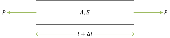
棒の引張り
ここで、\( l \) は棒の元の長さ、\( \Delta l \) は伸び。\( A \) は棒の断面積、\( E \) はヤング率(縦弾性係数とも)。\( P \) は荷重(引張荷重)
応力とひずみ
(ひずみは「歪」と漢字で書かれることも)
- 応力の定義\[ \sigma = \frac{P}{A} \]
- ひずみの定義\[ \varepsilon = \frac{\Delta l}{l} \]
フックの法則
\[ \sigma = E\varepsilon \]を仮定\[ \begin{align}
\sigma &= E\varepsilon \\
\frac{P}{A} &= E\frac{\Delta l}{l} \\
\Delta l &= \frac{Pl}{EA}
\end{align} \]
棒の伸び \( \Delta l \) は\[ \Delta l = \varepsilon l = \frac{Pl}{EA} \]となる
単位
| 量 | SI 単位 | 工学単位 |
|---|
| 荷重 P | N | kfg |
| 応力 σ | Pa
(N/m2) | kgf/mm2
SI 単位からの換算率 \( 1/(9.806\, 65\times 10^6) \) |
| ひずみ ε | 無次元 |
| ヤング率 E | Pa
(N/m2) | kgf/mm2 |
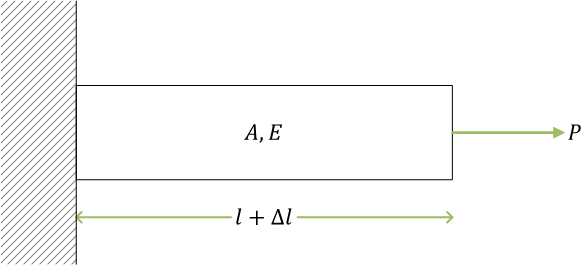
反力
(図でハッチングされているのは、剛体の壁)
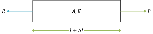
自由体図
ここで、\( R \) は反力(軸力)
力のつり合い。力のつり合い式\[ \begin{align} P - R &= 0 \\ R &= P \end{align} \](右向きの力を力の正の方向としている)
(材料力学では、力がつり合っている状態での材料の変形を考えている)
棒の伸び\[ \Delta l = \frac{Pl}{EA} \]
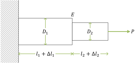
段付き丸棒(例題)
ここで、\( D_1 \) と \( D_2 \) は丸棒の直径。ヤング率 \( E \) は棒で一様(同一材料)とする
直径 \( D_1 \) の区間における応力、ひずみ、伸び\[ \sigma_1 = \frac{P}{A_1} = \frac{P}{\pi(D_1/2)^2} = \frac{4P}{\pi{D_1}^2}, \quad \varepsilon_1 = \frac{\sigma_1}{E} = \frac{4P}{E\pi{D_1}^2}, \quad \Delta l_1 = \varepsilon_1 l_1 = \frac{4P l_1}{E\pi{D_1}^2} \]
直径 \( D_2 \) の区間における応力、ひずみ、伸び\[ \sigma_2 = \frac{P}{A_2} = \frac{P}{\pi(D_2/2)^2} = \frac{4P}{\pi{D_2}^2}, \quad \varepsilon_2 = \frac{\sigma_2}{E} = \frac{4P}{E\pi{D_2}^2}, \quad \Delta l_2 = \varepsilon_2 l_2 = \frac{4P l_2}{E\pi{D_2}^2} \]
棒全体の伸び \( \Delta l \) は\[ \Delta l = \Delta l_1 + \Delta l_2 = \frac{4P l_1}{E\pi{D_1}^2} + \frac{4P l_2}{E\pi{D_2}^2} = \frac{4P}{E\pi} \left( \frac{l_1}{{D_1}^2} + \frac{l_2}{{D_2}^2} \right) \]それぞれの区間の伸びを足し合わせたものとなる
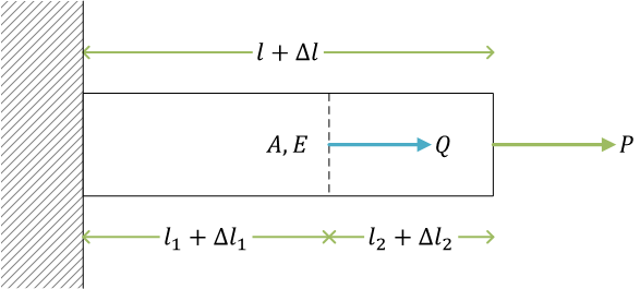
複数の荷重(例題)
ここで、荷重 \( Q \) も負荷されているとする
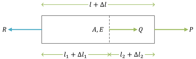
自由体図
\( R \) は反力
力のつり合い式\[ \begin{align}
P + Q - R &= 0 \\
R &= P + Q
\end{align} \]
それぞれの区間での伸び\[ \Delta l_1 = \frac{R l_1}{EA} = \frac{(P + Q)l_1}{EA} = \frac{P l_1 + Q l_1}{EA}, \quad \Delta l_2 = \frac{P l_2}{EA} \]
棒全体の伸び\[ \Delta l = \Delta l_1 + \Delta l_2 = \frac{P l_1 + Q l_1}{EA} + \frac{P l_2}{EA} = \frac{P(l_1 + l_2) + Q l_1}{EA} = \frac{P l + Q l_1}{EA} \]
∵ フックの法則は線形である(⇒ 重ね合わせの原理)
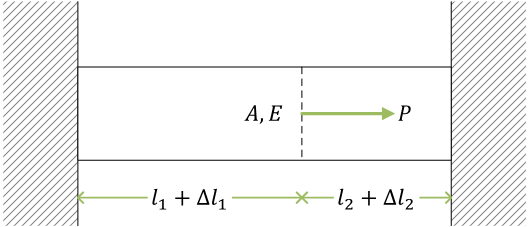
棒の不静定問題
(材料力学で、「力 → 応力 → ひずみ → 変形」という順に解くことができる問題のことは静定問題という)
力のつり合い式から反力を求めることができない(この問題は、静力学だけでは解くことができず、物体の変形を考慮しなければ解くことができない)
(不静定構造)
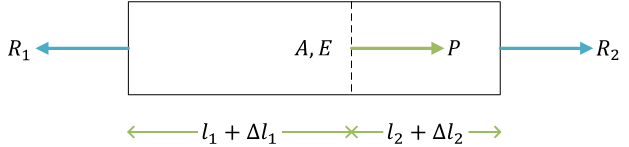
自由体図
ここで、\( R_1,\ R_2 \) は反力
力のつり合い式\[ \begin{align} P - R_1 + R_2 &= 0 \\ R_1 - R_2 &= P \end{align} \]\( R_1 \) と \( R_2 \) は未知数(不静定量)
それぞれの区間の応力、ひずみ、変形\[ \begin{gather}
\sigma_1 = \frac{ R_1 }{ A }, \quad \varepsilon_1 = \frac{ \sigma_1 }{ E } = \frac{ R_1 }{ EA }, \quad \Delta l_1 = \varepsilon_1 l_1 = \frac{ R_1 l_1 }{ EA } \\
\sigma_2 = \frac{ R_2 }{ A }, \quad \varepsilon_2 = \frac{ \sigma_2 }{ E } = \frac{ R_2 }{ EA }, \quad \Delta l_2 = \varepsilon_2 l_2 = \frac{ R_2 l_2 }{ EA }
\end{gather} \]
適合条件(伸びの条件)\[ \begin{align}
\Delta l_1 + \Delta l_2 &= 0 \\
\frac{ R_1 l_1 }{ EA } + \frac{ R_2 l_2 }{ EA } &= 0 \\
R_1 l_1 + R_2 l_2 &= 0
\end{align} \](この問題では、\( EA \) は共通因数なので消去することができる)
連立方程式\[ \left\{ \begin{align}
& R_1 - R_2 = P \\
& R_1 l_1 + R_2 l_2 = 0
\end{align} \right. \]を解く\[ \begin{gather} R_1 = \frac{l_2}{l_1 + l_2}P, \quad R_2 = -\frac{l_1}{l_1 + l_2}P \end{gather} \](反力 \( R_1,\ R_2 \) の符号より、棒の左側では引張り、右側では圧縮となっていることがわかる)
荷重 \( P \) の作用点における変位 \( \delta \)\[ \delta = \Delta l_1 = \frac{ R_1 l_1 }{ EA } \](座標系は、1次元、横軸右向きが正)
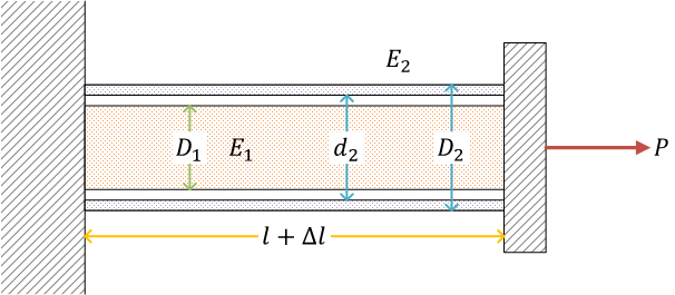
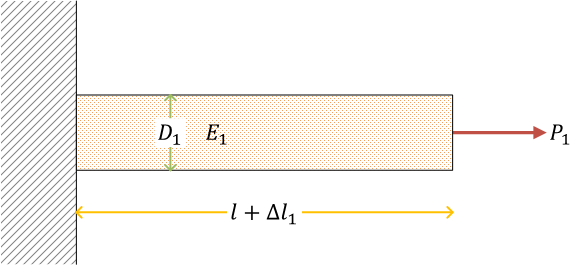
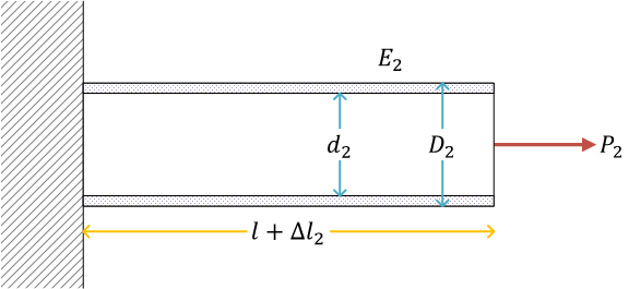
並列に接続された円柱と円筒(例題)
ここで、\( D_1 \) は中実丸棒の直径。\( d_2 \) は中空丸棒の内径、\( D_2 \) は中空丸棒の外径。\(E_1,\ E_2 \) はそれぞれの棒のヤング率
それぞれの棒の問題に分解して考える
中実の丸棒(円柱)
 |
中空の丸棒(円筒)
 |
荷重 \( P \) が、\( P_1,\ P_2 \) としてそれぞれの棒に配分される
力のつり合い式\[ \begin{align} P - P_1 - P_2 &= 0 \\ P_1 + P_2 &= P \end{align} \]\( P_1 \) と \( P_2 \) は未知数(不静定量)
中実丸棒の応力、ひずみ、伸び\[ \begin{gather}
\sigma_1 = \frac{P_1}{A_1} = \frac{4P_1}{\pi{D_1}^2}, \quad \varepsilon_1 = \frac{\sigma_1}{E_1} = \frac{4P_1}{E_1\pi{D_1}^2}, \quad \Delta l_1 = \varepsilon_1 l = \frac{4P_1 l}{E_1\pi{D_1}^2}
\end{gather} \]
中空丸棒の応力、ひずみ、伸び\[ \begin{gather}
\sigma_2 = \frac{P_2}{A_2} = \frac{4P_2}{\pi\left({D_2}^2 - {d_2}^2\right)}, \quad
\varepsilon_2 = \frac{\sigma_2}{E_2} = \frac{4P_2}{E_2\pi\left({D_2}^2 - {d_2}^2\right)}, \quad
\Delta l_2 = \varepsilon_2 l = \frac{4P_2 l}{E_2\pi\left({D_2}^2 - {d_2}^2\right)}
\end{gather} \]
適合条件(伸びの条件)\[ \begin{align}
\Delta l_1 &= \Delta l_2 \\
\Delta l_1 - \Delta l_2 &= 0 \\
\frac{4P_1 l}{E_1\pi{D_1}^2} - \frac{4P_2 l}{E_2\pi\left({D_2}^2 - {d_2}^2\right)} &= 0
\end{align} \]
連立方程式\[ \left\{ \begin{align}
& P_1 + P_2 = P \\
& \frac{4P_1 l}{E_1\pi{D_1}^2} - \frac{4P_2 l}{E_2\pi\left({D_2}^2 - {d_2}^2\right)} = 0
\end{align} \right. \]を解く\[
P_1 = \frac{E_1{D_1}^2}{E_1{D_1}^2 + E_2\left({D_2}^2 - {d_2}^2\right)}P, \quad
P_2 = \frac{E_2\left({D_2}^2 - {d_2}^2\right)}{E_1{D_1}^2 + E_2\left({D_2}^2 - {d_2}^2\right)}P
\]
伸び\[ \Delta l = \Delta l_1 = \Delta l_2 = \frac{4Pl}{\pi\left\{E_1{D_1}^2 + E_2\left({D_2}^2 - {d_2}^2\right)\right\}} \]
熱応力
いくつかの工業材料の線膨張係数(熱膨張係数とも)
| 材料 | 線膨張係数α[1/°C] |
|---|
| 鋼 | 9.6~11.6×10⁻⁶ |
| 鋳鉄 | 10~12×10-6 |
| ステンレス鋼 | 13.6×10⁻⁶ |
| 銅 | 18×10-6 |
| 黄銅(真ちゅう) | 19×10-6 |
| アルミニウム合金 | 23×10-6 |
| ポリカーボネート | 70×10-6 |
| シリコンゴム | 250~400×10-6 |
| セラミックス | 7~11×10-6 |
温度変化 \( \Delta T \) と棒の伸び \( \Delta l \) の関係式(仮定)\[ \begin{align}
\frac{\Delta l}{l} &= \alpha\Delta T \\
\Delta l &= l\alpha\Delta T
\end{align} \]ここで、\( \alpha \) が線膨張係数 [1/°C]
単位温度 1[°C] あたりのひずみ(単位長さあたりの伸び)を熱ひずみと呼ぶ\[ \varepsilon_\mathrm T = \frac{\Delta l}{l} = \alpha\Delta T \]\( \varepsilon_\mathrm T \) を熱ひずみ
- 温度変化は、絶対温度 [K] でも、摂氏 [°C] でも、同じ値になる
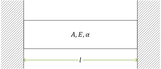
両端を固定された棒の熱応力(例題)
剛体断熱壁で棒を拘束
棒の温度を \( \Delta T \) だけ変化させる
(熱応力問題における)フックの法則\[ \sigma = E(\varepsilon - \varepsilon_\mathrm T) \]
- \( \bar{\varepsilon} \) を弾性ひずみ、\( \varepsilon_\mathrm T \) が熱ひずみ。足し合わせたものがひずみ \( \varepsilon = \bar\varepsilon + \varepsilon_\mathrm T \) となる
適合条件(伸びの条件)より \( \varepsilon = 0 \)\[ \sigma = E(0 - \varepsilon_\mathrm T) = -E\varepsilon_\mathrm T \]
よって、熱応力\[ \sigma = -E\varepsilon_\mathrm T = -E\alpha\Delta T \](引張りが正なので圧縮)が発生する
- 熱応力は、材料のヤング率 \( E \)、線膨張係数 \( \alpha \)、温度変化 \( \Delta T \) に比例する(棒の断面積 \( A \)、長さ \( l \) には無関係)
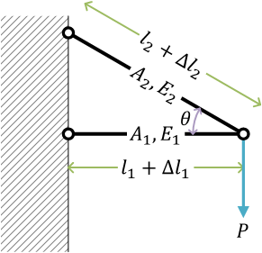
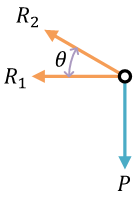
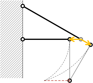
トラス構造
図で 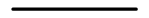 は棒の表示、
 は滑節。pin joint は回転を拘束しない
(そのため、トラスを構成するそれぞれの棒には引張り(圧縮)の力だけが作用する)
自由体図
ここで、\( R_1 \) と \( R_2 \) は、荷重 \( P \) が負荷される pin joint が、\( l_1 \) の棒から引張られる反力、\( l_2 \) の棒から引張られる反力
それぞれ\[ R_1 = -\frac{P}{\tan\theta}, \quad R_2 = \frac{P}{\sin\theta} \]
\( l_1 \) の棒と \( l_2 \) の棒の長さの関係 \[ l_2 = \frac{l_1}{\cos\theta} \]
\( l_1 \) の棒の伸び \( \Delta l_1 \)\[ \Delta l_1 = \frac{R_1 l_1}{EA} = -\frac{P l_1}{EA\tan\theta} \]
\( l_2 \) の棒の伸び \( \Delta l_2 \)\[ \Delta l_2 = \frac{R_2 l_2}{EA} = \frac{R_2}{EA}\frac{l_1}{\cos\theta} = \frac{P l_1}{EA\cos\theta\sin\theta} \]
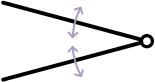
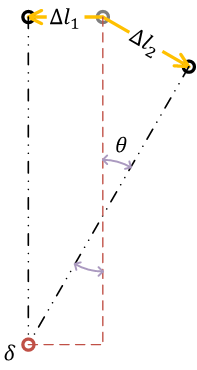
トラスの問題では、棒は回転ではなく、平行移動したと近似して考える
 | 近似 |  |
|---|
(材料力学では微小変形の問題を考えている(大変形問題は扱わない)。棒の長さに対して伸びは非常に小さいため、 近似的に、棒は、回転ではなく、平行移動をしたと考えることができる)
荷重点の変位 \( \delta \) を作図
幾何学より、水平方向変位 \( \delta_\mathrm{H} \)、鉛直方向変位 \( \delta_\mathrm{V} \) は\[ \begin{align}
& \delta_\mathrm{H} = \Delta l_1 \\
& \delta_\mathrm{V} = \frac{|\Delta l_1|}{\tan\theta} + \frac{\Delta l_2}{\sin\theta}
\end{align} \]となる
(座標系は、鉛直下向きを正)
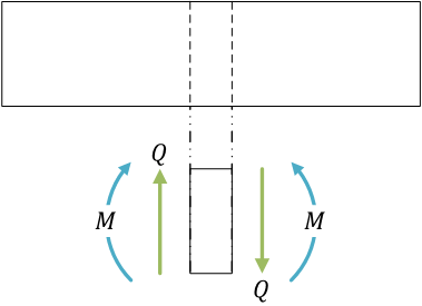
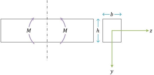
梁の曲げ
せん断力 \( Q \) と曲げモーメント \( M \) の正の方向
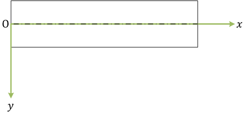
座標系の導入
X 軸は梁の中立面に一致させるようにとる。梁の左端が原点 O。座標系は、右手座標系。また、材料力学では、Y 軸を下向き正の方向にとることが多い
せん断力図と曲げモーメント図
それぞれ、shearing force diagram: SFD、bending moment diagram: BMD と略される
せん断力と曲げモーメントは、(導入した座標系で)x の関数になっている。せん断力を \( Q(x) \)、曲げモーメントを \( M(x) \)
せん断力は外力(荷重と反力)をすべて積分したものになっている。さらに、せん断力 \( Q(x) \) を積分すると、曲げモーメント \( M(x) \) になる《結論のみ。詳細は教科書など》
曲げ応力
\[ \sigma(y) = \frac{M(x)}{I}y \]ここで、\( I \) は断面二次モーメント【前方参照 ⇓】
最大曲げ応力 \( \sigma_\max \) は\[ \sigma^+_\max = \frac{M_\max}{Z_1}, \quad \sigma^-_\min = -\frac{M_\max}{Z_2} \]となる(\( ^+ \) の応力は引張り、\( ^- \) は圧縮)。ここで、\( Z \) は断面係数
《詳細は教科書など》
梁のたわみ
Bernoulli-Euler theory(平面保持の仮定とも)。Bernoulli-Euler 梁を考える
梁のたわみの微分方程式\[ \frac{d^2y(x)}{dx^2} = -\frac{M(x)}{EI} \]\( EI \) のことを曲げ剛性と呼ぶ(\( E \) はヤング率、\( I \) は断面二次モーメント【前方参照 ⇓】)
- 平面保持の仮定より、たわみ \( y(x) \) を微分して → たわみ角 \( \theta(x) \)\[ \theta(x) = \frac{dy(x)}{dx} \]
- さらに、たわみ角 \( \theta(x) \) を微分したものが → 曲率\[ \frac{d\theta(x)}{dx} = \frac{d^2 y(x)}{dx^2} \]
《結果のみ。導出、詳細は教科書など》
片持ちばり
(梁(はり)を「ばり」とも読む)片側を固定端、もう片側を自由端
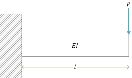
集中荷重を受ける片持ちばり(例題)
左端を固定端、右端を自由端
せん断力\[ Q(x) = P \]曲げモーメント\[ M(x) = -P(l - x) \]
SFD と BMD
作図に使用したプログラム
| Python |
|---|
import matplotlib.pyplot as plt

l = 1 # [m]
P = 1 # [N]

plt.clf(); plt.subplot(2, 1, 1)
plt.plot([0, 0, l, l], [0, P, P, 0], marker='.')
plt.plot([0, None, l], [0, None, 0], marker='.') # zero start, zero end
plt.title('SFD')
plt.xticks([0, l], [0, r'$ l $']); plt.yticks([0, P], [0, r'$ P $'])
plt.ylabel(r'$ Q $')

plt.subplot(2, 1, 2)
plt.plot([0, 0, l, l], [0, -P*l, 0, 0], marker='.')
plt.plot([0, None, l], [0, None, 0], marker='.') # zero start, zero end
plt.plot([0], [-P*l], marker='.', label=r'$ M_\max $')
plt.legend(loc='best')
plt.title('BMD')
plt.xticks([0, l], [0, r'$ l $']); plt.yticks([0, -P*l], [0, r'$ -Pl $'])
plt.xlabel(r'$ x $'); plt.ylabel(r'$ M $')

plt.savefig('fig_sfd_bmd.svg')
|
梁のたわみ曲線
\[ \begin{align}
\frac{d^2y(x)}{dx^2} &= -\frac{M(x)}{EI} = -\frac{-P(l -x )}{EI} \\
&= \frac{P}{EI}(l - x) \\
\frac{dy(x)}{dx} = \theta(x) &= \frac{P}{EI}\left(lx - \frac{1}{2}x^2\right) + \mathrm{C}_1 \\
y(x) &= \frac{P}{EI}\left(\frac{1}{2}lx^2 - \frac{1}{6}x^3\right) + \mathrm{C}_1 x + \mathrm{C}_2
\end{align}\](Maxima で検算)
| Maxima |
|---|
$ maxima

Maxima 5.43.2 http://maxima.sourceforge.net
using Lisp GNU Common Lisp (GCL) GCL 2.6.12
Distributed under the GNU Public License. See the file COPYING.
Dedicated to the memory of William Schelter.
The function bug_report() provides bug reporting information.
(%i1) M(x) := -P*(l - x);
(%o1)                        M(x) := (- P) (l - x)
(%i2) integrate('diff(y(x), x, 2) = -M(x)/(E*I), x);
                                              2
                                             x
                                    P (l x - --)
                        d                    2
(%o2)                   -- (y(x)) = ------------ + %c1
                        dx              E I
(%i3) integrate(%, x);
                                   2    3
                                l x    x
                             P (---- - --)
                                 2     6
(%o3)                 y(x) = ------------- + %c1 x + %c2
                                  E I
|
梁の境界条件より
- \( x = 0 \) において \( y = 0 \)
- また、\( x = 0 \) において \( \theta = 0 \)
積分定数は\[ \mathbf{C}_1 = 0, \quad \mathbf{C}_2 = 0 \]となる
よって\[ \theta(x) = \frac{P}{EI}\left(lx - \frac{1}{2}x^2\right), \quad y(x) = \frac{P}{EI}\left(\frac{1}{2}lx^2 - \frac{1}{6}x^3\right) \]
解を作図(たわみ(Y 軸)は、下向きを正としている)
作図に使用したプログラム
| Python | Maxima |
|---|
import numpy as np
import matplotlib.pyplot as plt

l = 1 # [m]
P = 1 # [N]
E = 1 # [Pa]
I = 1 # [m^4]

X = np.linspace(0, l, 1024)

plt.clf(); plt.subplot(2, 1, 1)
theta = [(P/(E*I))*(l*x - 1/2*x**2) for x in X]
plt.plot(X, theta)
assert theta[0] == 0
plt.plot([0], [0], marker='.') # boundary condition
assert round(theta[-1] - (P*l**2)/(2*E*I), 6) == 0
plt.plot(X[-1], theta[-1], marker='.', label=r'$ \theta_\max $')
plt.legend(loc='best')
plt.xticks([0, l], [0, r'$ l $']); plt.yticks([0, theta[-1]], [0, r'$ \frac{Pl^2}{2EI} $'])
plt.ylabel(r'$ \theta $')
plt.title('angle of deflection')

plt.subplot(2, 1, 2)
y = [(P/(E*I))*((1/2)*l*x**2 - (1/6)*x**3) for x in X]
plt.plot(X, y)
assert y[0] == 0
plt.plot([0], [0], marker='.') # boundary condition
assert round(y[-1] - (P*l**3)/(3*E*I), 6) == 0
plt.plot(X[-1], y[-1], marker='.', label=r'$ y_\max $')
plt.legend(loc='best')
plt.xticks([0, l], [0, r'$ l $']); plt.yticks([0, y[-1]], [0, r'$ \frac{Pl^3}{3EI} $'])
plt.xlabel(r'$ x $'); plt.ylabel(r'$ y $')
plt.title('deflection curve')

plt.gcf().get_axes()[0].invert_yaxis()
plt.gcf().get_axes()[1].invert_yaxis()

plt.savefig('fig_deflection.svg')
|
(%i1) M(x) := -P*(l - x);
(%o1)                        M(x) := (- P) (l - x)
(%i2) display2d: off;

(%o2) false
(%i3) integrate('diff(y(x), x, 2) = -M(x)/(E*I), x);

(%o3) 'diff(y(x),x,1) = (P*(l*x-x^2/2))/(E*I)+%c1
(%i4) integrate(%, x);

(%o4) y(x) = (P*((l*x^2)/2-x^3/6))/(E*I)+%c1*x+%c2
(%i5) ratsubst(l, x, (P*(l*x-x^2/2))/(E*I));

(%o5) (P*l^2)/(2*E*I)
(%i6) ratsubst(l, x, (P*((l*x^2)/2-x^3/6))/(E*I));

(%o6) (P*l^3)/(3*E*I)
|
∴ 片持ち梁のたわみ、たわみ角\[ y_\max = \frac{Pl^3}{3EI}, \quad \theta_\max = \frac{Pl^2}{2EI} \]
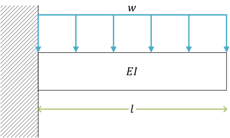
等分布荷重を受ける片持ちばり(例題)
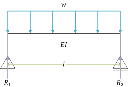
(等分布荷重 \( w \) の単位は [N/m])
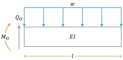
梁の自由体図。力のつり合い、モーメントのつり合い(材料力学では、力がつり合っている状態の問題を考えている)
図で、\( Q_\mathrm{O} \) と \( M_\mathrm{O} \) は、梁の左端(導入した座標系の原点)の剛体の壁と接している面で発生しているせん断力と曲げモーメント
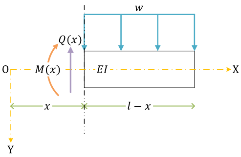
内力を考える。せん断力と曲げモーメントは、導入した座標系で \( x \) の関数になっている。それぞれ、\( Q(x) \) と \( M(x) \)
せん断力\[ Q(x) = w(l - x) \]
曲げモーメント\[ \begin{align}
M(x) &= -\left( \frac{l - x}{2} \times w(l - x) \right) \\
&= -\frac{w}{2}(l - x)^2
\end{align} \]
(Maxima で検算)曲げモーメントを微分するとせん断力になる
| Maxima |
|---|
(%i1) diff(M(x) = -w/2*(l - x)^2, x);
                             d
(%o1)                        -- (M(x)) = w (l - x)
                             dx
|
SFD と BMD
作図に使用したプログラム
| Python |
|---|
import matplotlib.pyplot as plt

l = 1 # [m]
w = 1 # [N/m]

plt.clf(); plt.subplot(2, 1, 1)
plt.plot([0, 0, l], [0, w*l, 0], marker='.')
plt.plot([0, None, l], [0, None, 0], marker='.') # zero start, zero end
plt.title('SFD')
plt.xticks([0, l], [0, r'$ l $']); plt.yticks([0, w*l], [0, r'$ wl $'])
plt.ylabel(r'$ Q $')

import numpy as np

plt.subplot(2, 1, 2)
X = np.linspace(0, l, 1024)
y = [-(w/2)*((l - x)**2) for x in X]
plt.plot(X, y)
plt.plot([0, 0, None, l], [0, -(w*(l**2))/2, None, 0], marker='.') # zero start, zero end
plt.plot([0], [-(w*(l**2))/2], marker='.', label=r'$ M_\max $')
plt.legend(loc='best')
plt.title('BMD')
plt.xticks([0, l], [0, r'$ l $']); plt.yticks([0, -(w*(l**2))/2], [0, r'$ -\frac{w l^2}{2} $'])
plt.xlabel(r'$ x $'); plt.ylabel(r'$ M $')

plt.savefig('fig_sfd_bmd2.svg')
|
梁のたわみの微分方程式を解く\[ \begin{align}
\frac{d^2 y(x)}{dx^2} &= -\frac{M(x)}{EI} \\
&= \frac{w}{2EI}(l - x)^2 \\
\frac{d y(x)}{dx} = \theta(x) &= \frac{w}{2EI}(\frac{x^3}{3} -lx^2 + l^2x) + \mathrm{C}_1 \\
y(x) &= \frac{w}{2EI}(\frac{x^4}{12} - \frac{lx^3}{3} + \frac{l^2x^2}{2}) + \mathrm{C}_1 + \mathrm{C}_2 \\
\end{align} \]
梁の境界条件より、積分定数を決定する
- \( x = 0 \) で \( \theta(x) = 0 \) となるので\[ \mathrm{C}_1 = 0 \]
- \( x = 0 \) で \( y(x) = 0 \) となるので\[ \mathrm{C}_2 = 0 \]
よって\[ \theta(x) = \frac{w}{2EI}(\frac{x^3}{3} -lx^2 + l^2x), \quad y(x) = \frac{w}{2EI}(\frac{x^4}{12} - \frac{lx^3}{3} + \frac{l^2x^2}{2}) \]
(Maxima で検算)
| Maxima |
|---|
(%i1) y(x) := (w/(2*E*I))*(x^4/12 - l*x^3/3 + l^2*x^2/2);
                                        4      3    2  2
                                 w     x    l x    l  x
(%o1)                 y(x) := (-----) (-- - ---- + -----)
                               2 E I   12    3       2
(%i2) \theta(x) = diff(y(x), x);
                                       3
                                      x       2    2
                                   w (-- - l x  + l  x)
                                      3
(%o2)                   theta(x) = --------------------
                                          2 E I
(%i3) 'diff('y(x), x, 2) = factor(diff(y(x), x, 2));
                             2                    2
                            d            w (x - l)
(%o3)                       --- (y(x)) = ----------
                              2            2 E I
                            dx
|
梁のたわみ曲線を作図
(たわみは、下向きを正)
作図に使用したプログラム
| Python | Maxima |
|---|
import numpy as np
import matplotlib.pyplot as plt

l = 1 # [m]
w = 1 # [N/m]
E = 1 # [Pa]
I = 1 # [m^4]

X = np.linspace(0, l, 1024)

plt.clf(); plt.subplot(2, 1, 1)
theta = [(w/(2*E*I))*(x**3/3 - l*x**2 + l**2*x) for x in X]
plt.plot(X, theta)
assert theta[0] == 0
plt.plot([0], [0], marker='.') # boundary condition
assert round(theta[-1] - (w*l**3)/(6*E*I), 6) == 0
plt.plot(X[-1], theta[-1], marker='.', label=r'$ \theta_\max $')
plt.legend(loc='best')
plt.xticks([0, l], [0, r'$ l $']); plt.yticks([0, theta[-1]], [0, r'$ \frac{wl^3}{6EI} $'])
plt.ylabel(r'$ \theta $')
plt.title('angle of deflection')

plt.subplot(2, 1, 2)
y = [(w/(2*E*I))*(x**4/12 - l*x**3/3 + l**2*x**2/2) for x in X]
plt.plot(X, y)
plt.plot([0], [0], marker='.') # boundary condition
assert round(y[-1] - (w*l**4)/(8*E*I), 6) == 0
plt.plot(X[-1], y[-1], marker='.', label=r'$ y_\max $')
plt.legend(loc='best')
plt.xticks([0, l], [0, r'$ l $']); plt.yticks([0, y[-1]], [0, r'$ \frac{wl^4}{8EI} $'])
plt.xlabel(r'$ x $'); plt.ylabel(r'$ y $')
plt.title('deflection curve')

plt.gcf().get_axes()[0].invert_yaxis()
plt.gcf().get_axes()[1].invert_yaxis()

plt.savefig('fig_deflection2.svg')
|
(%i1) display2d: off;

(%o1) false
(%i2) ratsubst(l, x, (w/(2*E*I))*(x^3/3 - l*x^2 + l^2*x));

(%o2) (l^3*w)/(6*E*I)
(%i3) ratsubst(l, x, (w/(2*E*I))*(x^4/12 - l*x^3/3 + l^2*x^2/2));

(%o3) (l^4*w)/(8*E*I)
|
∴ 梁のたわみ、たわみ角\[ y_\max = \frac{wl^4}{8EI}, \quad \theta_\max = \frac{wl^3}{6EI} \]
単純支持ばり
(梁を「ばり」とも読む。「両端支持ばり」ともいう)
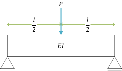
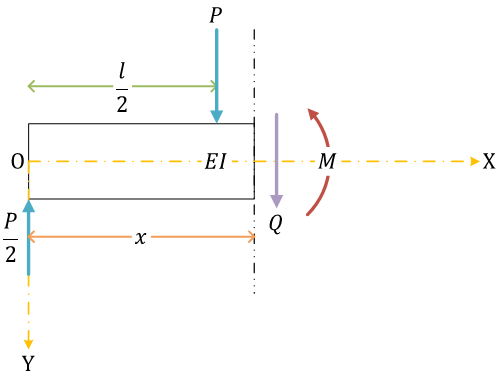
集中荷重を受ける単純支持ばり(例題)
(梁の3点曲げ)
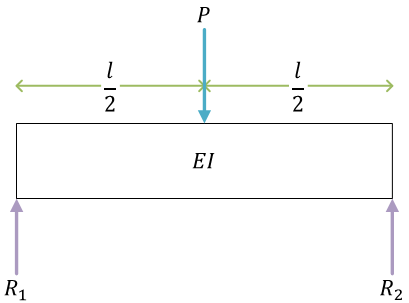
支点の反力を \( R_1 \)、\( R_2 \)
力のつり合い式\[ \begin{align}
P - R_1 - R_2 &= 0 \\
P &= R_1 + R_2
\end{align} \]
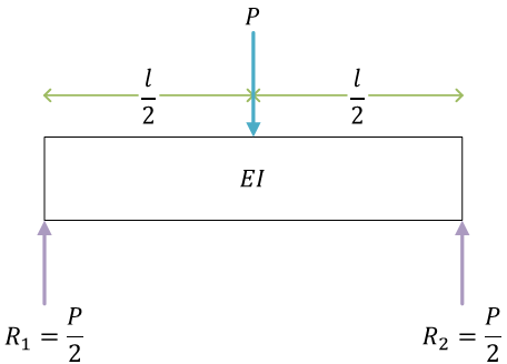
モーメントのつり合い式\[ \begin{align}
\frac{l}{2}\times P - l\times R_2 &= 0 \\
R_2 &= \frac{P}{2}
\end{align} \](梁の左端を回転中心)
|
(モーメントのつり合いを考えるときには、どの点まわりで考えてもよい。結果は同じになる)梁の右端の点まわり \[ \begin{align}
l\times R_1 - \frac{l}{2}\times P &= 0 \\
R_1 &= \frac{P}{2}
\end{align} \] 梁の中心、集中荷重 \( P \) が負荷されている荷重点まわり\[ \begin{align}
\frac{l}{2}\times R_1 - \frac{l}{2}\times R_2 &= 0 \\
R_1 &= R_2 \end{align}
\]
|
反力 \( R_1 \)、\( R_2 \) を、与えられている荷重 \( P \) で記述する
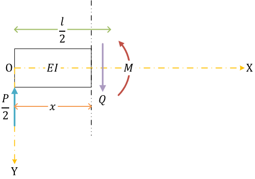
せん断力と曲げモーメント。集中荷重 \( P \) より左側、右側で場合分けして考える
| \[ 0 \leq x \leq \frac{l}{2} \] | \[ \frac{l}{2} \leq x \leq l \] |
|---|
|
|
せん断力\[ Q(x) = \frac{P}{2} \]曲げモーメント\[ M(x) = \frac{P}{2}x \] |
せん断力\[ \begin{align}
Q(x) + P &= \frac{P}{2} \\
Q(x) &= -\frac{P}{2}
\end{align} \]曲げモーメント\[ \begin{align}
M(x) + P(x - \frac{l}{2}) &= \frac{P}{2}x \\
M(x) &= -\frac{P}{2}x + \frac{Pl}{2} \\
&= \frac{P}{2}(l - x)
\end{align}\] |
式を整理。せん断力\[ Q(x) = \begin{cases}
\frac{P}{2} & (0 \leq x \leq \frac{l}{2}) \\
-\frac{P}{2} & (\frac{l}{2} \leq x \leq l)
\end{cases} \]曲げモーメント\[ M(x) = \begin{cases}
\frac{P}{2}x & (0 \leq x \leq \frac{l}{2}) \\
\frac{P}{2}(l - x) & (\frac{l}{2} \leq x \leq l)
\end{cases} \]
SFD と BMD
作図に使用したプログラム
| Python |
|---|
import matplotlib.pyplot as plt

l = 1 # [m]
P = 1 # [N]

plt.clf(); plt.subplot(2, 1, 1)
plt.plot([0, 0, l/2, l/2, l, l], [0, P/2, P/2, -P/2, -P/2, 0], marker='.')
plt.plot([0, None, l], [0, None, 0], marker='.') # zero start, zero end
plt.title('SFD')
plt.xticks([0, l], [0, r'$ l $']); plt.yticks([-P/2, 0, P/2], [r'$ -\frac{P}{2} $', 0, r'$ \frac{P}{2} $'])
plt.ylabel(r'$ Q $')

plt.subplot(2, 1, 2)
plt.plot([0, l/2, l], [0, P*l/4, 0], marker='.')
plt.plot([0, None, l], [0, None, 0], marker='.') # zero start, zero end
plt.plot([l/2], [P*l/4], marker='.', label=r'$ M_\max $')
plt.legend(loc='best')
plt.title('BMD')
plt.xticks([0, l/2, l], [0, r'$ \frac{l}{2} $', r'$ l $']); plt.yticks([0, P*l/4], [0, r'$ \frac{Pl}{4} $'])
plt.xlabel(r'$ x $'); plt.ylabel(r'$ M $')

plt.savefig('fig_sfd_bmd3.svg')
|
梁のたわみの微分方程式。同様に、集中荷重 \( P \) の右側、左側で梁を分けて、別々に微分方程式を立てる
| \[ 0 \leq x \leq \frac{l}{2} \] | | \[ \frac{l}{2} \leq x \leq l \] |
|---|
梁の左側部分のたわみを \( y_1 \) とする\[ \begin{align}
\frac{d^2 y_1(x)}{dx^2} &= -\frac{M(x)}{EI} \\
&= -\frac{P}{2EI}x
\end{align} \] |
\[ \quad \] |
梁の右側部分のたわみを \( y_2 \) とする\[ \begin{align}
\frac{d^2 y_2(x)}{dx^2} &= -\frac{M(x)}{EI} \\
&= -\frac{P}{2EI}(l - x)
\end{align} \] |
梁のたわみの微分方程式を解く(以下、Maxima による記号計算)
| Maxima |
|---|
(%i1) M(x) := P/2*x;
                                          P
(%o1)                            M(x) := (-) x
                                          2
(%i2) ode1: 'diff(y_1(x), x, 2) = -M(x)/(E*I);
                             2
                            d                 P x
(%o2)                       --- (y_1(x)) = - -----
                              2              2 E I
                            dx
(%i3) M(x) := P/2*(l - x);
                                       P
(%o3)                         M(x) := (-) (l - x)
                                       2
(%i4) ode2: 'diff(y_2(x), x, 2) = -M(x)/(E*I);
                           2
                          d                P (l - x)
(%o4)                     --- (y_2(x)) = - ---------
                            2                2 E I
                          dx
(%i5) eqn1: integrate(ode1, x);
                                                  2
                           d                   P x
(%o5)                      -- (y_1(x)) = %c1 - -----
                           dx                  4 E I
(%i6) eqn2: integrate(eqn1, x);
                                       3
                                    P x
(%o6)                  y_1(x) = (- ------) + %c1 x + %c2
                                   12 E I
(%i7) eqn3: integrate(ode2, x);
                                                     2
                                                    x
                                           P (l x - --)
                       d                            2
(%o7)                  -- (y_2(x)) = %c3 - ------------
                       dx                     2 E I
(%i8) eqn4: integrate(eqn3, x);
                                     2    3
                                  l x    x
                               P (---- - --)
                                   2     6
(%o8)              y_2(x) = (- -------------) + %c3 x + %c4
                                   2 E I
|
境界条件を使って積分定数を求める。梁の支持条件より
- \( x = 0 \) で \( y_1 = 0 \)
- また、\( x = l \) で \( y_2 = 0 \)
積分定数を求める
| Maxima(つづき) |
|---|
(%i9) c2: rhs(solve(ratsubst(0, x, 0 = rhs(eqn2)), %c2)[1]);
(%o9)                                  0
(%i10) c4: rhs(solve(ratsubst(l, x, 0 = rhs(eqn4)), %c4)[1]);
                                 3
                              P l  - 6 %c3 E I l
(%o10)                        ------------------
                                    6 E I
|
さらに、梁のたわみ曲線の連続性より(連続条件)
- \( x = \frac{l}{2} \) で \( \frac{d y_1(x)}{dx} = \frac{d y_2(x)}{dx} \)\[ \left.\frac{d y_1(x)}{dx}\right|_{x = \frac{l}{2}} = \left.\frac{d y_2(x)}{dx}\right|_{x = \frac{l}{2}} \]
- また、\( x = \frac{l}{2} \) で \( y_1 = y_2 \)
連立方程式を解く
| Maxima(つづき) |
|---|
(%i11) eqn5: ratsubst(l/2, x, rhs(eqn1) = rhs(eqn3));
                       2                       2
                    P l  - 16 %c1 E I     3 P l  - 16 %c3 E I
(%o11)            - ----------------- = - -------------------
                         16 E I                 16 E I
(%i12) eqn6: ratsubst(l/2, x, ratsubst(c2, %c2, rhs(eqn2)) = ratsubst(c4, %c4, rhs(eqn4)));
                     3                        3
                  P l  - 48 %c1 E I l   11 P l  - 48 %c3 E I l
(%o12)          - ------------------- = ----------------------
                        96 E I                  96 E I
(%i13) ans: solve([eqn5, eqn6], [%c1, %c3]);
                                    2              2
                                 P l          3 P l
(%o13)                  [[%c1 = ------, %c3 = ------]]
                                16 E I        16 E I
(%i14) c1: rhs(ans[1][1]);
                                        2
                                     P l
(%o14)                              ------
                                    16 E I
(%i15) c3: rhs(ans[1][2]);
                                         2
                                    3 P l
(%o15)                              ------
                                    16 E I
|
求まった解
| Maxima(つづき) |
|---|
(%i16) eqn7: \\theta_1(x) = rhs(ratsubst(c1, %c1, eqn1));
                                              2      2
                                         4 P x  - P l
(%o16)                   \theta_1(x) = - -------------
                                            16 E I
(%i17) eqn8: \\theta_2(x) = rhs(ratsubst(c3, %c3, eqn3));
                                       2                  2
                                  4 P x  - 8 P l x + 3 P l
(%o17)              \theta_2(x) = -------------------------
                                           16 E I
(%i18) eqn9: ratsubst(c1, %c1, ratsubst(c2, %c2, eqn2));
                                         3        2
                                    4 P x  - 3 P l  x
(%o18)                   y_1(x) = - -----------------
                                         48 E I
(%i19) eqn10: ratsubst(c3, %c3, ratsubst(c4, %c4, eqn4));
                               3           2        2        3
                          4 P x  - 12 P l x  + 9 P l  x - P l
(%o19)           y_2(x) = ------------------------------------
                                         48 E I
(%i20) tex(eqn7);
\[ {\it \theta}_{1}\left(x\right)=-{{4\,P\,x^2-P\,l^2}\over{16\,E\,I}} \]
(%i21) tex(eqn8);
\[ {\it \theta}_{2}\left(x\right)={{4\,P\,x^2-8\,P\,l\,x+3\,P\,l^2}\over{16\,E\,I}} \]
(%i22) tex(eqn9);
\[ y_{1}\left(x\right)=-{{4\,P\,x^3-3\,P\,l^2\,x}\over{48\,E\,I}} \]
(%i23) tex(eqn10);
\[ y_{2}\left(x\right)={{4\,P\,x^3-12\,P\,l\,x^2+9\,P\,l^2\,x-P\,l^3}\over{48\,E\,I}} \]
|
梁の代表的な位置 \( x = (0,\ 1,\ \frac{l}{2}) \)(梁の左端、右端、梁の真ん中)で、たわみ \( y_1,\ y_2 \) とたわみ角 \( \theta_1,\ \theta_2 \)(添え字 \( _{1,\ 2} \) は、集中荷重 \( P \) の左側、右側)を計算して、解に問題がないことを確認
| Maxima(つづき) |
|---|
(%i24) ratsubst(0, x, eqn9);
(%o24)                            y_1(0) = 0
(%i25) ratsubst(l, x, eqn10);
(%o25)                            y_2(l) = 0
(%i26) ratsubst(l/2, x, eqn9);
                                             3
                                    l     P l
(%o26)                          y_1(-) = ------
                                    2    48 E I
(%i27) ratsubst(l/2, x, eqn10);
                                             3
                                    l     P l
(%o27)                          y_2(-) = ------
                                    2    48 E I
|
(%i28) ratsubst(0, x, eqn7);
                                               2
                                            P l
(%o28)                       \theta_1(0) = ------
                                           16 E I
(%i29) ratsubst(l, x, eqn8);
                                                2
                                             P l
(%o29)                      \theta_2(l) = - ------
                                            16 E I
(%i30) ratsubst(l/2, x, eqn7);
                                         l
(%o30)                          \theta_1(-) = 0
                                         2
(%i31) ratsubst(l/2, x, eqn8);
                                         l
(%o31)                          \theta_2(-) = 0
                                         2
|
梁のたわみ曲線
作図プログラム
| Maxima(つづき) |
|---|
(%i32) fortran(rhs(eqn7));
      -((4*P*x**2-P*l**2)/(E*I))/1.6E+1
(%o32)                               done
(%i33) fortran(rhs(eqn8));
      ((4*P*x**2-8*P*l*x+3*P*l**2)/(E*I))/1.6E+1
(%o33)                               done
(%i34) fortran(rhs(eqn9));
      -((4*P*x**3-3*P*l**2*x)/(E*I))/4.8E+1
(%o34)                               done
(%i35) fortran(rhs(eqn10));
      ((4*P*x**3-12*P*l*x**2+9*P*l**2*x-P*l**3)/(E*I))/4.8E+1
(%o35)                               done
(%i36) fortran(rhs(%o28));
      ((P*l**2)/(E*I))/1.6E+1
(%o36)                               done
(%i37) fortran(rhs(%o29));
      -((P*l**2)/(E*I))/1.6E+1
(%o37)                               done
(%i38) fortran(rhs(%o26));
      ((P*l**3)/(E*I))/4.8E+1
(%o38)                               done
|
| Python |
|---|
import numpy as np
import matplotlib as mpl
mpl.use('Agg')
import matplotlib.pyplot as plt

P = 1 # [N]
l = 1 # [m]
E = 1 # [Pa]
I = 1 # [m^4]

X = [np.linspace(0, l/2, 1024), np.linspace(l/2, l, 1024)]

def theta_1(x):
    return -((4*P*x**2-P*l**2)/(E*I))/1.6E+1

def theta_1_max():
    return ((P*l**2)/(E*I))/1.6E+1

assert theta_1(0) == theta_1_max()

def theta_2(x):
    return ((4*P*x**2-8*P*l*x+3*P*l**2)/(E*I))/1.6E+1

assert theta_1(l/2) == theta_2(l/2)

def theta_2_max():
    return -((P*l**2)/(E*I))/1.6E+1

assert theta_2(l) == theta_2_max()
assert theta_1_max() == -theta_2_max()

plt.clf(); plt.subplot(2, 1, 1)
theta = [[theta_1(x) for x in X[0]], [theta_2(x) for x in X[1]]]
assert theta[0][-1] == theta[1][0]
plt.plot(X[0], theta[0], color='tab:blue'); plt.plot(X[1], theta[1], color='tab:blue')
assert theta[0][0] == theta_1_max() and theta[1][-1] == theta_2_max()
plt.plot([0, None, l], [theta_1_max(), None, theta_2_max()], marker='.', color='tab:green', label=r'$ \theta_\max $')
plt.legend(loc='best')
plt.xticks([0, l], [0, r'$ l $']);
plt.yticks([theta_2_max(), 0, theta_1_max()], [r'$ -\frac{Pl^2}{16EI} $', 0, r'$ \frac{Pl^2}{16EI} $'])
plt.ylabel(r'$ \theta $')
plt.title('angle of deflection')

def y_1(x):
    return -((4*P*x**3-3*P*l**2*x)/(E*I))/4.8E+1

def y_2(x):
    return ((4*P*x**3-12*P*l*x**2+9*P*l**2*x-P*l**3)/(E*I))/4.8E+1

assert y_1(l/2) == y_2(l/2)

def y_max():
    return ((P*l**3)/(E*I))/4.8E+1

assert y_1(l/2) == y_max()
assert y_2(l/2) == y_max()

plt.subplot(2, 1, 2)
y = [[y_1(x) for x in X[0]], [y_2(x) for x in X[1]]]
assert y[0][-1] == y[1][0]
plt.plot(X[0], y[0], color='tab:blue'); plt.plot(X[1], y[1], color='tab:blue')
assert y[0][0] == 0 and y[1][-1] == 0
plt.plot([0, None, l], [0, None, 0], marker='.', color='tab:orange') # boundary condition
assert y[0][-1] == y_max() and y[1][0] == y_max()
plt.plot([l/2], [y_max()], marker='.', color='tab:green', label=r'$ y_\max $')
plt.legend(loc='best')
plt.xticks([0, l/2, l], [0, r'$ \frac{l}{2} $', r'$ l $']); plt.yticks([0, y_max()], [0, r'$ \frac{Pl^3}{48EI} $'])
plt.xlabel(r'$ x $'); plt.ylabel(r'$ y $')
plt.title('deflection curve')

plt.gcf().get_axes()[0].invert_yaxis()
plt.gcf().get_axes()[1].invert_yaxis()

plt.savefig('fig_deflection3.svg')
|
∴ 梁のたわみ、たわみ角\[ y_\max = \frac{Pl^3}{48EI}, \quad \theta_\max = \pm\frac{Pl^2}{16EI} \]
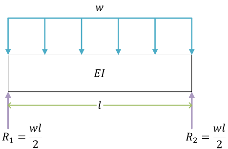
等分布荷重を受ける単純支持ばり(例題)
力のつり合い式\[ \begin{align}
\int_0^l w\, dx - R_1 - R_2 &= 0 \\
[wx]_0^l - R_1 - R_2 &= 0 \\
wl - R_1 - R_2 &= 0 \\
R_1 + R_2 &= wl
\end{align} \]
モーメントのつり合い式\[ \begin{align}
\int_0^l x\times w\, dx - l\times R_2 &= 0 \\
\left[\frac{wx^2}{2}\right]_0^l - l\times R_2 &= 0 \\
\frac{wl^2}{2} - l\times R_2 &= 0 \\
lR_2 &= \frac{wl^2}{2} \\
R_2 &= \frac{wl}{2}
\end{align} \](梁の左端まわり)
よって\[ R_1 = R_2 = \frac{wl}{2} \]
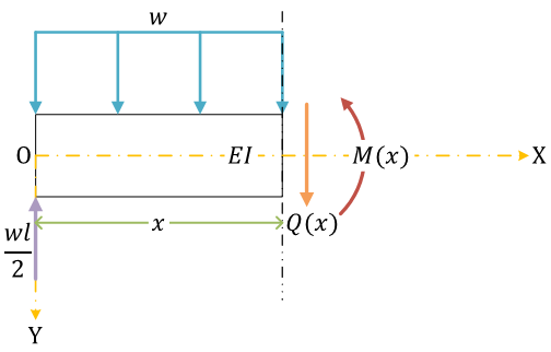
自由体図、反力
内力を考える
せん断力\[ \begin{align}
wx + Q(x) -\frac{wl}{2} &= 0 \\
wx + Q(x) &= \frac{wl}{2} \\
Q(x) &= -wx + \frac{wl}{2}
\end{align} \]
曲げモーメント\[ \begin{align}
\frac{x}{2}\times wx + M(x) - x\times\frac{wl}{2} &= 0 \\
\frac{w}{2}x^2 + M(x) &= \frac{wl}{2}x \\
M(x) &= -\frac{w}{2}x^2 + \frac{wl}{2}x
\end{align} \](Maxima で検算)
| Maxima |
|---|
(%i1) diff(M(x) = -w/2*x^2 + w*l/2*x, x);
                             d           l w
(%o1)                        -- (M(x)) = --- - w x
                             dx           2
|
(曲げモーメントを微分するとせん断力になる)
SFD と BMD
作図プログラム
| Maxima |
|---|
(%i1) M(x) := -w/2*x^2 + w*l/2*x;
                                   - w   2    w l
(%o1)                     M(x) := (---) x  + (---) x
                                    2          2
(%i2) M(l/2);
                                      2
                                     l  w
(%o2)                                ----
                                      8
|
| Python |
|---|
import matplotlib
matplotlib.use('Agg')
import matplotlib.pyplot as plt

w = 1 # [N/m]
l = 1 # [m]

plt.clf(); plt.subplot(2, 1, 1)
plt.plot([0, 0, l, l], [0, w*l/2, -w*l/2, 0], marker='.')
plt.title('SFD')
plt.plot([0, None, l], [0, None, 0], marker='.') # zero start, zero end
plt.xticks([0, l], [0, r'$ l $']); plt.yticks([-w*l/2, 0, w*l/2], [r'$ -\frac{wl}{2} $', 0, r'$ \frac{wl}{2} $'])
plt.ylabel(r'$ Q $')

import numpy as np

def M_max():
    return w*l**2/8

plt.subplot(2, 1, 2)
X = np.linspace(0, l, 1024)
y = [-w/2*x**2 + w*l/2*x for x in X]
plt.plot(X, y)
plt.plot([0, None, l], [0, None, 0], marker='.') # zero start, zero end
plt.plot([l/2], [M_max()], marker='.', label=r'$ M_\max $')
plt.legend(loc='best')
plt.title('BMD')
plt.xticks([0, l/2, l], [0, r'$ \frac{l}{2} $', r'$ l $']); plt.yticks([0, M_max()], [0, r'$ \frac{wl^2}{8} $'])
plt.xlabel(r'$ x $'); plt.ylabel(r'$ M $')

plt.savefig('fig_sfd_bmd4.svg')
|
梁のたわみの微分方程式\[ \begin{align}
\frac{d^2 y(x)}{dx^2} &= -\frac{M(x)}{EI} = \frac{w}{2EI}x^2 - \frac{wl}{2EI}x \\
&= \frac{w}{2EI}(x^2 - lx)
\end{align} \]
(Maxima による記号計算)
| Maxima |
|---|
(%i1) M(x) := -w/2*(x^2 - l*x);
                                    - w    2
(%o1)                      M(x) := (---) (x  - l x)
                                     2
(%i2) eqn1: integrate('diff('y(x), x, 2) = -M(x)/(E*I), x);
                                        3      2
                                       x    l x
                                    w (-- - ----)
                        d              3     2
(%o2)                   -- (y(x)) = ------------- + %c1
                        dx              2 E I
(%i3) eqn2: integrate(eqn1, x);
                                 4      3
                                x    l x
                             w (-- - ----)
                                12    6
(%o3)                 y(x) = ------------- + %c1 x + %c2
                                 2 E I
|
境界条件
- \( x = 0 \) で \( y = 0 \)
- また、\( x = l \) でも \( y = 0 \)
より
| Maxima(つづき) |
|---|
(%i4) c2: rhs(solve(0 = ratsubst(0, x, rhs(eqn2)), %c2)[1]);
(%o4)                                  0
(%i5) c1: rhs(solve(0 = ratsubst(l, x, ratsubst(c2, %c2, rhs(eqn2))), %c1)[1]);
                                      3
                                     l  w
(%o5)                               ------
                                    24 E I
(%i6) eqn3: \\theta(x) = ratsubst(c1, %c1, rhs(eqn1));
                                      3          2    3
                                 4 w x  - 6 l w x  + l  w
(%o6)                \theta(x) = ------------------------
                                          24 E I
(%i7) eqn4: ratsubst(c1, %c1, ratsubst(c2, %c2, eqn2));
                                  4          3    3
                               w x  - 2 l w x  + l  w x
(%o7)                   y(x) = ------------------------
                                        24 E I
(%i8) tex(eqn3);
\[ {\it \theta}\left(x\right)={{4\,w\,x^3-6\,l\,w\,x^2+l^3\,w}\over{24\,E\,I}} \]
(%i9) tex(eqn4);
\[ y\left(x\right)={{w\,x^4-2\,l\,w\,x^3+l^3\,w\,x}\over{24\,E\,I}} \]
|
梁のたわみ曲線
作図プログラム
| Maxima(つづき) |
|---|
(%i10) fortran(rhs(eqn3));
      ((4*w*x**3-6*l*w*x**2+l**3*w)/(E*I))/2.4E+1
(%o10)                               done
(%i11) ratsubst(0, x, eqn3); fortran(rhs(%));
                                            3
                                           l  w
(%o11)                        \theta(0) = ------
                                          24 E I
      ((l**3*w)/(E*I))/2.4E+1
(%o12)                               done
(%i13) ratsubst(l, x, eqn3); fortran(rhs(%));
                                             3
                                            l  w
(%o13)                       \theta(l) = - ------
                                           24 E I
      -((l**3*w)/(E*I))/2.4E+1
(%o14)                               done
(%i15) fortran(rhs(eqn4));
      ((w*x**4-2*l*w*x**3+l**3*w*x)/(E*I))/2.4E+1
(%o15)                               done
(%i16) ratsubst(l/2, x, eqn4); fortran(rhs(%));
                                          4
                                  l    5 l  w
(%o16)                          y(-) = -------
                                  2    384 E I
      (5.0E+0*l**4*w)/(3.84E+2*E*I)
(%o17)                               done
|
| Python |
|---|
import numpy as np
import matplotlib as mpl
mpl.use('Agg')
import matplotlib.pyplot as plt

w = 1 # [N/m]
l = 1 # [m]
E = 1 # [Pa]
I = 1 # [m^4]

X = np.linspace(0, l, 1024)

def theta(x):
    return ((4*w*x**3-6*l*w*x**2+l**3*w)/(E*I))/2.4E+1

def theta_max_1():
    return ((l**3*w)/(E*I))/2.4E+1

def theta_max_2():
    return -((l**3*w)/(E*I))/2.4E+1

assert theta(0) == theta_max_1() and theta(l) == theta_max_2()
assert theta_max_1() == -theta_max_2()

plt.clf(); plt.subplot(2, 1, 1)
plt.plot(X, [theta(x) for x in X])
plt.plot([0, None, l], [theta_max_1(), None, theta_max_2()], marker='.', color='tab:green', label=r'$ \theta_\max $')
plt.legend(loc='best')
plt.xticks([0, l], [0, r'$ l $'])
plt.yticks([theta_max_2(), 0, theta_max_1()], [r'$ -\frac{wl^3}{24EI} $', 0, r'$ \frac{wl^3}{24EI} $'])
plt.ylabel(r'$ \theta $')
plt.title('angle of deflection')

def y(x):
    return ((w*x**4-2*l*w*x**3+l**3*w*x)/(E*I))/2.4E+1

assert y(0) == 0 and y(l) == 0

def y_max():
    return (5.0E+0*l**4*w)/(3.84E+2*E*I)

assert y(l/2) == y_max()

plt.subplot(2, 1, 2)
plt.plot(X, [y(x) for x in X])
plt.plot([0, None, l], [0, None, 0], marker='.') # boundary condition
plt.plot([l/2], y_max(), marker='.', label=r'$ y_\max $')
plt.legend(loc='best')
plt.xticks([0, l/2, l], [0, r'$ \frac{l}{2} $', r'$ l $'])
plt.yticks([0, y_max()], [0, r'$ \frac{5wl^4}{384EI} $'])
plt.xlabel(r'$ x $'); plt.ylabel(r'$ y $')
plt.title('deflection curve')

plt.gcf().get_axes()[0].invert_yaxis()
plt.gcf().get_axes()[1].invert_yaxis()

plt.savefig('fig_deflection4.svg')
|
∴ 梁のたわみ、たわみ角\[ y_\max = \frac{5wl^4}{384EI}, \quad \theta_\max = \pm\frac{wl^3}{24EI} \]
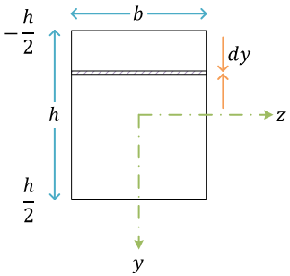
長方形断面
座標系は、z 軸を中立軸に一致するようにとる
断面二次モーメント \( I \) は、断面形状と中立軸の位置により定まる。また、\( I \) の単位は mm4
長方形断面の \( I \)\[ \begin{align}
I &= \int_A y^2\, dA = \int_{-\frac{h}{2}}^{\frac{h}{2}}by^2\, dy = b\int_{-\frac{h}{2}}^{\frac{h}{2}}y^2\, dy = b\left[\frac{y^3}{3}\right]_{-\frac{h}{2}}^{\frac{h}{2}} \\
&= \frac{bh^3}{12}
\end{align} \]
断面の形状が、円形断面ならば\[ I = \frac{\pi D^4}{64} \](円形断面の断面二次モーメントの導出や、その他の断面形状については、教科書など)《積み残し》
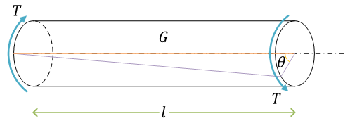
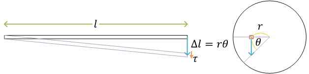
軸のねじり
(丸棒について)
\( T \) は、ねじりモーメント。または、ねじりモーメントのことをトルクという。また、\( \theta \) をねじれ角
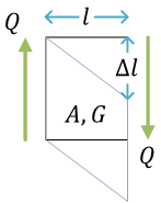
せん断
- せん断応力、せん断ひずみ\[ \tau = \frac{Q}{A}, \quad \gamma = \frac{\Delta l}{l} \]
- せん断弾性係数 \( G \)(せん断におけるフックの法則)\[ \tau = G\gamma \] (\( G \) は、横弾性係数とも)
ねじれ角を求める
せん断ひずみ\[ \gamma = \frac{\Delta l}{l} = \frac{r\theta}{l} \]せん断応力\[ \tau = G\gamma = G\frac{r\theta}{l} \]
軸まわりのモーメントのつり合いより、せん断力による軸まわりのモーメントの合計がねじりモーメント(トルク)になる\[ \begin{align}
T &= \int_A r\times\tau\, dA = \int_0^{2\pi} \!\!\! \int_0^\frac{D}{2} G\frac{r^2}{l}\theta r\, drd\theta = \frac{G}{l}\theta\int_0^{2\pi} \!\!\! \int_0^\frac{D}{2} r^3\, drd\theta \\
&= \frac{G}{l}\theta\left[2\pi\frac{r^4}{4} \right]_0^\frac{D}{2} \\
&= \frac{G}{l}\theta\frac{\pi D^4}{32}
\end{align} \]
ここで、\( \frac{\pi D^4}{32} \) を \( I_\mathrm{p} \) とおいて式を整理\[ T = \frac{G I_\mathrm{p}}{l}\theta \]\( I_\mathrm{p} \) のことを断面二次極モーメント
重積分と極座標系(復習)
\[ dA = dxdy = |J|drd\theta = rdrd\theta \] 極座標\[ \left\{\begin{align}
&x = r\cos\theta \\
&y = r\sin\theta
\end{align}\right. \] ヤコビアン\[ \quad |J| = \begin{vmatrix} \frac{\partial x}{\partial r} & \frac{\partial x}{\partial\theta} \\ \frac{\partial y}{\partial r} & \frac{\partial y}{\partial\theta} \end{vmatrix} = \begin{vmatrix} \cos\theta & -r\sin\theta \\ \sin\theta & r\cos\theta \end{vmatrix} = r\left(\cos^2\theta + \sin^2\theta\right) = r \quad \]
|
よって、ねじれ角 \( \theta \) は\[ \theta = \frac{T l}{G I_\mathrm{p}} \]となる
- \( G I_\mathrm{p} \) をねじり剛性という
- 単位長さあたりのねじれ角 \( \frac{\theta}{l} = \frac{T}{G I_\mathrm{p}} \) のことを、比ねじれ角という
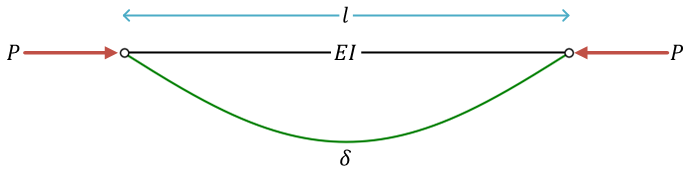
柱の座屈
(柱は、長柱(ちょうちゅう)とも)
弾性座屈(Euler's buckling とも)
(\( EI \) は、曲げ剛性)
座屈荷重\[ P_\mathrm{c} = \left(\frac{\pi}{l}\right)^2 EI \]
(詳細は教科書など)《座屈については、積み残し》
Rahmen 構造
《積み残し》
教科書
© 2023 Tadakazu Nagai