現代制御理論(modern control theory)

永井 忠一 2022.7.31

状態方程式(state equation)

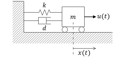
質量、ばね、ダンパーからなる力学系

\( m \) : 質量 \( k \) : ばね定数 \( d \) : ダンパー係数（粘性摩擦係数）

運動方程式（力のつりあい）\[ \begin{align} m\ddot{x} + d\dot{x} + kx &= f \\ \ddot{x} &= -\frac{d}{m}\dot{x} - \frac{k}{m}x + \frac{1}{m}f \end{align} \]

状態変数(state variable)

位置（変位）と速度を選ぶ\[ \boldsymbol{x}(t) = \begin{pmatrix} x \\ \dot{x} \end{pmatrix} \]（状態変数の各要素は独立であることが必要）

状態方程式\[ \frac{d}{dt}\boldsymbol{x}(t) = \begin{pmatrix} \dot{x} \\ \ddot{x} \end{pmatrix} = \begin{pmatrix} 0 & 1 \\ -\frac{k}{m} & -\frac{d}{m} \end{pmatrix}\begin{pmatrix} x \\ \dot{x} \end{pmatrix} + \begin{pmatrix} 0 \\ \frac{1}{m} \end{pmatrix}f \]（行列微分方程式。２階の線形微分方程式が、ベクトル \( \boldsymbol{x}(t) \) に関する１階の微分方程式として書ける）

出力方程式（観測方程式とも）\[ \boldsymbol y(t) = \begin{pmatrix} 1 & 0 \end{pmatrix}\begin{pmatrix} x \\ \dot x \end{pmatrix} \]（出力方程式は、代数方程式）

状態空間表現(state space representation)

状態方程式と出力方程式をあわせて\[ \left\{ \begin{align} \dot{\boldsymbol x}(t) &= \begin{pmatrix} 0 & 1 \\ -\frac{k}{m} & -\frac{d}{m} \end{pmatrix}\boldsymbol x(t) + \begin{pmatrix} 0 \\ \frac{1}{m} \end{pmatrix}f \\ \boldsymbol y(t) &= \begin{pmatrix} 1 & 0 \end{pmatrix}\boldsymbol x(t) \end{align} \right. \]状態空間表現\[ \boldsymbol u(t) \longrightarrow \boxed{\boldsymbol x(t)} \longrightarrow \boldsymbol y(t) \]入力（古典制御では操作量）\( \boldsymbol u(t) \in \mathbb R^p \)、出力（古典制御では制御量）\( \boldsymbol y(t) \in \mathbb R^q \)。そして、（システムの内部）状態 \( \boldsymbol x(t) \in \mathbb R^n \)

（cf. 古典制御（伝達関数）による表現）

n 次元の状態変数 \( \boldsymbol x \) を持つため、n 次元システム(n-dimensional system)とも呼ばれる\[ \boldsymbol x(t) = \begin{bmatrix} x_1(t) \\ x_2(t) \\ \vdots \\ x_n(t) \end{bmatrix} \in \mathbb R^n,\quad \boldsymbol u(t) = \begin{bmatrix} u_1(t) \\ u_2(t) \\ \vdots \\ u_p(t) \end{bmatrix} \in \mathbb R^p,\quad \boldsymbol y(t) = \begin{bmatrix} y_1(t) \\ y_2(t) \\ \vdots \\ y_q(t) \end{bmatrix} \in \mathbb R^q \]

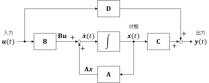
状態空間表現の一般形\[ \left\{ \begin{align} \dot{\boldsymbol x}(t) &= \mathbf A\boldsymbol x(t) + \mathbf B\boldsymbol u(t) \\ \boldsymbol y(t) &= \mathbf C\boldsymbol x(t) + \mathbf D\boldsymbol u(t) \end{align} \right. \]システム行列 \( \mathbf A \in \mathbb R^{n\times n} \)、入力行列 \( \mathbf B \in \mathbb R^{n\times p} \)。出力行列 \( \mathbf C \in \mathbb R^{q\times n} \)、それから \( \mathbf D \in \mathbb R^{q\times p} \)

（システム \( \mathbf \Sigma \) と呼ぶこともある）システム \( (\mathbf A,\, \mathbf B,\, \mathbf C,\, \mathbf D) \)\[ \begin{bmatrix} \mathbf A \in \mathbb R^{n\times n} & \mathbf B \in \mathbb R^{n\times p} \\ \mathbf C \in \mathbb R^{q\times n} & \mathbf D \in \mathbb R^{q\times p} \end{bmatrix} \]

\( \mathbf D\boldsymbol u(t) \) は直達項(feedthrouth term)。入力 \( \boldsymbol u(t) \) が、出力 \( \boldsymbol y(t) \) へダイナミクスを経由しないで現れる（機械系の例では、機構学や静力学）\[ \boldsymbol u(t) \longrightarrow \boxed{\mathbf D} \longrightarrow \boldsymbol y(t) \]\( \mathbf D = \mathbf 0 \) の場合\[ \left\{ \begin{align} \dot{\boldsymbol x}(t) &= \mathbf A\boldsymbol x(t) + \mathbf B\boldsymbol u(t) \\ \boldsymbol y(t) &= \mathbf C\boldsymbol x(t) \end{align} \right. \]

状態空間表現によって表されるシステムのブロック線図

（数学）

\( \dot{\boldsymbol x}(t) = \mathbf A\boldsymbol x(t) + \mathbf B\boldsymbol u(t) \) の解\[ \boldsymbol x(t) = e^{\mathbf A(t - t_0)}\boldsymbol x(t_0) + \int_{t_0}^{t}e^{\mathbf A(t - \tau)}\mathbf B\boldsymbol u(\tau)\, d\tau \]

確認のため、上記の式を時間 \( t \) で微分

$ maxima

Maxima 5.43.2 http://maxima.sourceforge.net
using Lisp GNU Common Lisp (GCL) GCL 2.6.12
Distributed under the GNU Public License. See the file COPYING.
Dedicated to the memory of William Schelter.
The function bug_report() provides bug reporting information.
(%i1) 'diff(x(t), t) = diff(exp(A.(t - t_0)).x(t_0) + integrate(exp(A.(t - \\tau)).B.u(\\tau), \\tau, t_0, t), t)$

(%i2) tex(%);

Maxima の記号計算結果を、手作業で式を整理\[ \begin{align} \dot{\boldsymbol x}(t) &= \mathbf A e^{\mathbf A(t - t_0)}\boldsymbol x(t_0) + \int_{t_0}^{t}\mathbf A e^{\mathbf A(t - \tau)}\mathbf B\boldsymbol u(\tau)\, d\tau + \mathbf B\boldsymbol u(t) \\ &= \mathbf A e^{\mathbf A(t - t_0)}\boldsymbol x(t_0) + \mathbf A\int_{t_0}^{t}e^{\mathbf A(t - \tau)}\mathbf B\boldsymbol u(\tau)\, d\tau + \mathbf B\boldsymbol u(t) \\ &= \mathbf A\left\{ e^{\mathbf A(t - t_0)}\boldsymbol x(t_0) + \int_{t_0}^{t}e^{\mathbf A(t - \tau)}\mathbf B\boldsymbol u(\tau)\, d\tau \right\} + \mathbf B\boldsymbol u(t) \\ &= \mathbf A\boldsymbol x(t) + \mathbf B\boldsymbol u(t) \end{align}\]（∴ \( \boldsymbol x(t) \) が、状態方程式の解となっている）

\( t_0 = 0 \) ならば（時刻 \( t_0 \) が \( 0 \) の場合の式の形）\[ \boldsymbol x(t) = e^{\mathbf A t}\boldsymbol x_0 + \int_{0}^{t}e^{\mathbf A(t - \tau)}\mathbf B u(\tau)\, d\tau \]

（線形なので、重ね合わせの理(principle of superposition)が成り立つ。右辺第１項は自由応答(free response)（初期値応答）、第２項は外力（制御では入力）に対する応答の項。右辺第２項は、状態遷移行列と \( \mathbf B\boldsymbol u \)（入力）の畳み込み積分(convolution)となる）

状態方程式の解\[ \begin{align} \dot{\boldsymbol x}(t) = \mathbf A\boldsymbol x(t) + \mathbf B\boldsymbol u(t) \quad \xrightarrow{\mathcal L} \quad s\boldsymbol X(s) - \boldsymbol x_0 &= \mathbf A\boldsymbol X(s) + \mathbf B\boldsymbol U(s) \\ s\boldsymbol X(s) - \mathbf A\boldsymbol X(s) &= \boldsymbol x_0 + \mathbf B\boldsymbol U(s) \\ s\mathbf I\boldsymbol X(s) - \mathbf A\boldsymbol X(s) &= \boldsymbol x_0 + \mathbf B\boldsymbol U(s) \\ (s\mathbf I - \mathbf A)\boldsymbol X(s) &= \boldsymbol x_0 + \mathbf B\boldsymbol U(s) \\ \boldsymbol x(t) = e^{\mathbf A t}\boldsymbol x_0 + \int_0^t e^{\mathbf A(t - \tau)}\mathbf B\boldsymbol u(\tau)\, d\tau \quad \xleftarrow{\mathcal L^{-1}} \quad \boldsymbol X(s) &= (s\mathbf I - \mathbf A)^{-1}\boldsymbol x_0 + (s\mathbf I - \mathbf A)^{-1}\mathbf B\boldsymbol U(s) \end{align} \]

状態方程式をラプラス変換\[ \begin{align} \dot{\boldsymbol x}(t) = \mathbf A\boldsymbol x(t) + \mathbf B\boldsymbol u(t) \quad \xrightarrow{\mathcal L} \quad s\boldsymbol X(s) - \boldsymbol x_0 &= \mathbf A\boldsymbol X(s) + \mathbf B\boldsymbol U(s) \\ s\boldsymbol X(s) - \mathbf A\boldsymbol X(s) &= \boldsymbol x_0 + \mathbf B\boldsymbol U(s) \\ s\mathbf I\boldsymbol X(s) - \mathbf A\boldsymbol X(s) &= \boldsymbol x_0 + \mathbf B\boldsymbol U(s) \\ \boxed{(s\mathbf I - \mathbf A)}\boldsymbol X(s) &= \boldsymbol x_0 + \mathbf B\boldsymbol U(s) \\ \boldsymbol X(s) &= \boxed{(s\mathbf I - \mathbf A)^{-1}}\boldsymbol x_0 + \boxed{(s\mathbf I - \mathbf A)^{-1}}\mathbf B\boldsymbol U(s) \end{align} \]（もし、\( (s\mathbf I - \mathbf A) \) が逆行列を持つならば）\( s \) 領域で、\( \boldsymbol X(s) \) について解くことができる

時間領域の解。右辺第１項\[ \boldsymbol x(t) = \boxed{e^{\mathbf A t}\boldsymbol x_0} + \int_0^t e^{\mathbf A(t - \tau)}\mathbf B\boldsymbol u(\tau)\, d\tau \quad \xleftarrow{\mathcal L^{-1}} \quad \boldsymbol X(s) = \boxed{(s\mathbf I - \mathbf A)^{-1}\boldsymbol x_0} + (s\mathbf I - \mathbf A)^{-1}\mathbf B\boldsymbol U(s) \]の逆ラプラス変換\[ e^{\mathbf A t} = \mathcal L^{-1}\left[ (s\mathbf I - \mathbf A)^{-1} \right] \]（cf. （スカラー関数の）指数関数のラプラス逆変換）

右辺第２項\[ \boldsymbol x(t) = e^{\mathbf A t}\boldsymbol x_0 + \boxed{\int_0^t e^{\mathbf A(t - \tau)}\mathbf B\boldsymbol u(\tau)\, d\tau} \quad \xleftarrow{\mathcal L^{-1}} \quad \boldsymbol X(s) = (s\mathbf I - \mathbf A)^{-1}\boldsymbol x_0 + \boxed{(s\mathbf I - \mathbf A)^{-1}\mathbf B\boldsymbol U(s)} \]の逆ラプラス変換\[ \begin{align} \int_0^t e^{\mathbf A(t -\tau)}\mathbf B\boldsymbol u(\tau)\, d\tau &= \mathcal L^{-1}\left[ (s\mathbf I - \boldsymbol A)^{-1}\mathbf B\boldsymbol U(s) \right] \\ &= \mathcal L^{-1}\left[ \left( (s\mathbf I - \boldsymbol A)^{-1} \right) \left( \mathbf B\boldsymbol U(s) \right) \right] \\ &= \mathcal L^{-1}\left[ \mathcal L\left[ e^{\mathbf A t}\right]\mathcal L\left[ \mathbf B\boldsymbol u(t) \right] \right] \end{align} \]（２つのラプラス変換を掛け合わせたものの逆ラプラス変換は、畳み込み積分）

\[ \therefore ~ \boldsymbol x(t) = e^{\mathbf A t}\boldsymbol x_0 + \int_0^t e^{\mathbf A(t - \tau)}\mathbf B\boldsymbol u(\tau)\, d\tau \]

出力方程式（観測方程式）の解（\( \boldsymbol x(t) \) に行列 \( \mathbf C \) を（左から）掛けたもの）\[ \begin{align} \boldsymbol x(t) &= e^{\mathbf A t}\boldsymbol x_0 + \int_0^t e^{\mathbf A(t - \tau)}\mathbf B\boldsymbol u(\tau)\, d\tau \\ \boldsymbol y(t) = \mathbf C\boldsymbol x(t) &= \mathbf C e^{\mathbf A t}\boldsymbol x_0 + \int_0^t \mathbf C e^{\mathbf A(t - \tau)}\mathbf B\boldsymbol u(\tau)\, d\tau \end{align} \]

（直達項がある場合には\[ \boldsymbol y(t) = \mathbf Ce^{\mathbf At}\boldsymbol x_0 + \int_0^t\mathbf Ce^{\mathbf A(t-\tau)}\mathbf B\boldsymbol u(\tau)\, d\tau + \mathbf D\boldsymbol u(t) \]となる）

状態遷移行列

無限級数展開、逆ラプラス変換により求められる（式再掲載）\[ \begin{align} e^{\mathbf{A}t} &= \mathbf{I} + \frac{1}{1!}\mathbf{A}t + \frac{1}{2!}\mathbf{A}^{2}t^2 + \frac{1}{3!}\mathbf{A}^{3}t^{3} + \cdots = \sum_{k = 0}^{\infty}\frac{1}{k!}\mathbf{A}^{k}t^{k} \\ e^{\mathbf{A}t} &= \mathcal{L}^{-1}\left[ (s\mathbf{I} - \mathbf{A})^{-1} \right] \end{align} \]

時間応答

（上記システムにパラメータと初期値をあたえて時間応答を求める。）システム

\[ \begin{gather} m = 1, \quad k = 5, \quad d = 6 \\ \mathbf A = \begin{pmatrix} 0 & 1 \\ -\frac{k}{m} & -\frac{d}{m} \end{pmatrix} = \begin{pmatrix} 0 & 1 \\ -5 & -6 \end{pmatrix}, \quad \mathbf B = \begin{pmatrix} 0 \\ \frac{1}{m} \end{pmatrix} = \begin{pmatrix} 0 \\ 1 \end{pmatrix} \end{gather}\]

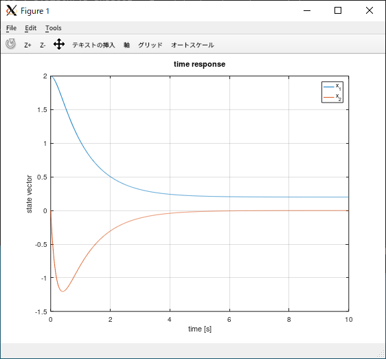
状態方程式\[ \begin{gather} \dot{\boldsymbol x}(t) = \begin{pmatrix} 0 & 1 \\ -5 & -6 \end{pmatrix}\boldsymbol x(t) + \begin{pmatrix} 0 \\ 1 \end{pmatrix}u(t) \\ \boldsymbol x(0) = \boldsymbol x_0 = \begin{pmatrix} 2 \\ 0 \end{pmatrix}, \quad u = 1, \quad t \ge 0 \end{gather} \]

状態変数\[ \boldsymbol x(t) = \begin{pmatrix} x_1 = x(t) \\ x_2 = \dot x(t) \end{pmatrix} \]

（状態変数 \( \boldsymbol x(t) \) は直接観測できるものとする。つまり、\( \boldsymbol y(t) = \begin{pmatrix} 1 & 0 \\ 0 & 1 \end{pmatrix}\boldsymbol x(t) \)）

Maxima による記号計算

(%i1) A: matrix([0, 1], [-5, -6]);
                                 [  0    1  ]
(%o1)                            [          ]
                                 [ - 5  - 6 ]
(%i2) eAt: genmatrix(lambda([i, j], ilt((invert(s*ident(2) - A))[i, j], s, t)), 2, 2); /* state transition matrix */
                  [      - t     - 5 t      - t     - 5 t  ]
                  [  5 %e      %e         %e      %e       ]
                  [  ------- - -------    ----- - -------  ]
                  [     4         4         4        4     ]
(%o2)             [                                        ]
                  [     - 5 t       - t      - 5 t     - t ]
                  [ 5 %e        5 %e     5 %e        %e    ]
                  [ --------- - -------  --------- - ----- ]
                  [     4          4         4         4   ]
(%i3) tex(exp('A*t) = %);

(%i4) x0: matrix([2], [0]);
                                     [ 2 ]
(%o4)                                [   ]
                                     [ 0 ]
(%i5) Bu: matrix([0], [1]);
                                     [ 0 ]
(%o5)                                [   ]
                                     [ 1 ]
(%i6) eAt.x0 + integrate(subst(t - \\tau, t, eAt.Bu), \\tau, 0, t);
           [      - 5 t      4 t                - t     - 5 t      ]
           [    %e      (5 %e    - 1)       5 %e      %e         1 ]
           [ (- ---------------------) + 2 (------- - -------) + - ]
           [             20                    4         4       5 ]
(%o6)      [                                                       ]
           [       - 5 t    4 t               - 5 t       - t      ]
           [     %e      (%e    - 1)      5 %e        5 %e         ]
           [     ------------------- + 2 (--------- - -------)     ]
           [              4                   4          4         ]
(%i7) x: ratsimp(%);
                     [   - 5 t      5 t        4 t      ]
                     [ %e      (4 %e    + 45 %e    - 9) ]
                     [ -------------------------------- ]
                     [                20                ]
(%o7)                [                                  ]
                     [         - 5 t      4 t           ]
                     [       %e      (9 %e    - 9)      ]
                     [     - ---------------------      ]
                     [                 4                ]
(%i8) tex('x(t) = %);

状態方程式の解のグラフ

(%i9) fortran(x);

      x(1,1) = (exp(-5*t)*(4*exp(5*t)+45*exp(4*t)-9))/2.0E+1
      x(2,1) = -(exp(-5*t)*(9*exp(4*t)-9))/4.0E+0

$ octave --no-gui
GNU Octave, version 5.2.0
Copyright (C) 2020 John W. Eaton and others.
This is free software; see the source code for copying conditions.
There is ABSOLUTELY NO WARRANTY; not even for MERCHANTABILITY or
FITNESS FOR A PARTICULAR PURPOSE.  For details, type 'warranty'.

Octave was configured for "x86_64-pc-linux-gnu".

Additional information about Octave is available at https://www.octave.org.

Please contribute if you find this software useful.
For more information, visit https://www.octave.org/get-involved.html

Read https://www.octave.org/bugs.html to learn how to submit bug reports.
For information about changes from previous versions, type 'news'.

octave:1> type -q time_response.m
clear all

if false
  my_time = 0:0.01:10;
else
  my_time = linspace(0, 10, 1024);
end

i = 1;
for t = my_time
  x_1(i) = (exp(-5*t)*(4*exp(5*t)+45*exp(4*t)-9))/2.0E+1;
  x_2(i) = -(exp(-5*t)*(9*exp(4*t)-9))/4.0E+0;
  i = i + 1;
end

clf
plot(my_time, x_1)
hold
plot(my_time, x_2)
grid on
legend("x_1", "x_2")
xlabel("time [s]")
ylabel("state vector")
title("time response")

if false
  print("time_response.png", "-dpng");
end

octave:2> time_response

手計算による再計算。状態遷移行列\[ e^{\mathbf At} = \mathcal L^{-1}\left[ (s\mathbf I - \mathbf A)^{-1} \right] = \begin{pmatrix} -\frac{1}{4}e^{-5t} + \frac{5}{4}e^{-t} & -\frac{1}{4}e^{-5t} + \frac{1}{4}e^{-t} \\ \frac{5}{4}e^{-5t} - \frac{5}{4}e^{-t} & \frac{5}{4}e^{-5t} - \frac{1}{4}e^{-t} \end{pmatrix} \] 状態方程式の解\[ \begin{align} \boldsymbol x(t) &= e^{\mathbf A t}\boldsymbol x_0 + \int_0^t e^{\mathbf A(t - \tau)}\mathbf B u(\tau)\, d\tau \\ &= \begin{bmatrix} -\frac{1}{4}e^{-5t} + \frac{5}{4}e^{-t} & -\frac{1}{4}e^{-5t} + \frac{1}{4}e^{-t} \\ \frac{5}{4}e^{-5t} - \frac{5}{4}e^{-t} & \frac{5}{4}e^{-5t} - \frac{1}{4}e^{-t} \end{bmatrix}\begin{pmatrix} 2 \\ 0 \end{pmatrix} + \int_0^t\begin{bmatrix} -\frac{1}{4}e^{-5(t - \tau)} + \frac{5}{4}e^{-(t - \tau)} & -\frac{1}{4}e^{-5(t - \tau)} + \frac{1}{4}e^{-(t - \tau)} \\ \frac{5}{4}e^{-5(t - \tau)} - \frac{5}{4}e^{-(t - \tau)} & \frac{5}{4}e^{-5(t - \tau)} - \frac{1}{4}e^{-(t - \tau)} \end{bmatrix}\begin{pmatrix} 0 \\ 1 \end{pmatrix}\, d\tau \\ &= \begin{bmatrix} -\frac{1}{2}e^{-5t} + \frac{5}{2}e^{-t} \\ \frac{5}{2}e^{-5t} - \frac{5}{2}e^{-t} \end{bmatrix} + \int_0^t\begin{bmatrix} -\frac{1}{4}e^{-5(t - \tau)} + \frac{1}{4}e^{-(t - \tau)} \\ \frac{5}{4}e^{-5(t - \tau)} - \frac{1}{4}e^{-(t - \tau)} \end{bmatrix}\, d\tau \\ &= \begin{bmatrix} -\frac{1}{2}e^{-5t} + \frac{5}{2}e^{-t} \\ \frac{5}{2}e^{-5t} - \frac{5}{2}e^{-t} \end{bmatrix} + \begin{bmatrix} -\frac{1}{20}e^{-5(t - t)} + \frac{1}{4}e^{-(t - t)} \\ \frac{1}{4}e^{-5(t - t)} - \frac{1}{4}e^{-(t - t)} \end{bmatrix} - \begin{bmatrix} -\frac{1}{20}e^{-5t} + \frac{1}{4}e^{-t} \\ \frac{1}{4}e^{-5t} - \frac{1}{4}e^{-t} \end{bmatrix} \\ &= \begin{bmatrix} -\frac{1}{2}e^{-5t} + \frac{5}{2}e^{-t} \\ \frac{5}{2}e^{-5t} - \frac{5}{2}e^{-t} \end{bmatrix} + \begin{bmatrix} -\frac{1}{20}e^0 + \frac{1}{4}e^0 \\ \frac{1}{4}e^0 - \frac{1}{4}e^0 \end{bmatrix} - \begin{bmatrix} -\frac{1}{20}e^{-5t} + \frac{1}{4}e^{-t} \\ \frac{1}{4}e^{-5t} - \frac{1}{4}e^{-t} \end{bmatrix} \\ &= \begin{bmatrix} -\frac{1}{2}e^{-5t} + \frac{5}{2}e^{-t} \\ \frac{5}{2}e^{-5t} - \frac{5}{2}e^{-t} \end{bmatrix} + \begin{bmatrix} -\frac{1}{20} + \frac{1}{4} \\ \frac{1}{4} - \frac{1}{4} \end{bmatrix} - \begin{bmatrix} -\frac{1}{20}e^{-5t} + \frac{1}{4}e^{-t} \\ \frac{1}{4}e^{-5t} - \frac{1}{4}e^{-t} \end{bmatrix} \\ &= \begin{bmatrix} -\frac{1}{2}e^{-5t} + \frac{5}{2}e^{-t} \\ \frac{5}{2}e^{-5t} - \frac{5}{2}e^{-t} \end{bmatrix} + \begin{bmatrix} \frac{1}{5} \\ 0 \end{bmatrix} - \begin{bmatrix} -\frac{1}{20}e^{-5t} + \frac{1}{4}e^{-t} \\ \frac{1}{4}e^{-5t} - \frac{1}{4}e^{-t} \end{bmatrix} \\ &= \begin{bmatrix} -\frac{9}{20}e^{-5t} + \frac{9}{4}e^{-t} + \frac{1}{5} \\ \frac{9}{4}e^{-5t} - \frac{9}{4}e^{-t} \end{bmatrix} \end{align} \]Maxima の答えと検算

(%i1) eAt: genmatrix(lambda([i, j], ilt((invert(s*ident(2) - matrix([0, 1], [-5, -6])))[i, j], s, t)), 2, 2)$

(%i2) eAt - matrix([-(1/4)*%e^(-5*t) + (5/4)*%e^(-t), -(1/4)*%e^(-5*t) + (1/4)*%e^(-t)], [(5/4)*%e^(-5*t) - (5/4)*%e^(-t), (5/4)*%e^(-5*t) - (1/4)*%e^(-t)]);
                                   [ 0  0 ]
(%o2)                              [      ]
                                   [ 0  0 ]
(%i3) x: eAt.matrix([2], [0]) + integrate(subst(t - \\tau, t, eAt.matrix([0], [1])), \\tau, 0, t)$

(%i4) ratsimp(x - matrix([-(9/20)*%e^(-5*t) + (9/4)*%e^(-t) + (1/5)], [(9/4)*%e^(-5*t) - (9/4)*%e^(-t)]));
                                     [ 0 ]
(%o4)                                [   ]
                                     [ 0 ]

lsim() 関数による状態方程式の解

octave:1> type -q time_response_lsim.m
pkg load control

clear all
A = [0 1; -5 -6]
B = [0; 1]
C = eye(2)
D = zeros(2, 1)

x0 = [2; 0]

t = linspace(0, 10, 1024);
u = ones(1, length(t));

x = lsim(ss(A, B, C, D), u, t, x0);

if true
  clf
  plot(t, x(:,1))
  hold
  plot(t, x(:,2))
  grid on
  legend("x_1", "x_2")
  xlabel("time [s]")
  ylabel("state vector")
  title("time response")
end

if false
  print("time_response_lsim.png", "-dpng");
end

octave:2> format compact
octave:3> time_response_lsim
A =
   0   1
  -5  -6

B =
   0
   1

C =
Diagonal Matrix
   1   0
   0   1

D =
   0
   0

x0 =
   2
   0

Octave の control パッケージのインストール（私の環境では Linux apt）

$ sudo apt install octave-control

位相面(phase plane)

上記システムの状態変数\[ \boldsymbol x(t) = \begin{pmatrix} x_1(t) = x(t) \\ x_2(t) = \dot x(t) \end{pmatrix} \]の初期値 \( \boldsymbol x_0 \) を乱数で適当に決定して、状態方程式の解を可視化（相図(phase portrait)）

横軸を位置 \( x_1 = x \)、縦軸を速度 \( x_2 = \dot x \)

状態変数の初期値 \( \boldsymbol x_0 \) を変数のままとした状態方程式の解を求めて描画

(%i1) A: matrix([0, 1], [-5, -6]);
                                 [  0    1  ]
(%o1)                            [          ]
                                 [ - 5  - 6 ]
(%i2) eAt: genmatrix(lambda([i, j], ilt((invert(s*ident(2) - A))[i, j], s, t)), 2, 2);
                  [      - t     - 5 t      - t     - 5 t  ]
                  [  5 %e      %e         %e      %e       ]
                  [  ------- - -------    ----- - -------  ]
                  [     4         4         4        4     ]
(%o2)             [                                        ]
                  [     - 5 t       - t      - 5 t     - t ]
                  [ 5 %e        5 %e     5 %e        %e    ]
                  [ --------- - -------  --------- - ----- ]
                  [     4          4         4         4   ]
(%i3) x0: matrix([x_1], [x_2]);
                                    [ x_1 ]
(%o3)                               [     ]
                                    [ x_2 ]
(%i4) Bu: matrix([0], [1]);
                                     [ 0 ]
(%o4)                                [   ]
                                     [ 1 ]
(%i5) x: ratsimp(eAt.x0 + integrate(subst(t - \\tau, t, eAt.Bu), \\tau, 0, t));
                 - 5 t       4 t                  4 t                5 t
(%o5) matrix([(%e      ((5 %e    - 5) x_2 + (25 %e    - 5) x_1 + 4 %e
       4 t
 - 5 %e    + 1))/20], 
     - 5 t     4 t                 4 t              4 t
   %e      ((%e    - 5) x_2 + (5 %e    - 5) x_1 - %e    + 1)
[- ---------------------------------------------------------])
                               4
(%i6) fortran(x);

$ ipython3 
Python 3.8.10 (default, Jun 22 2022, 20:18:18) 
Type 'copyright', 'credits' or 'license' for more information
IPython 7.13.0 -- An enhanced Interactive Python. Type '?' for help.

In [1]: %cat phase_plane.py
from math import exp
import numpy as np
import matplotlib.pyplot as plt

if False:
    my_time = np.arange(0, 10, 0.01)
else:
    my_time = np.linspace(0, 10, 1024*16)

np.random.seed(0)
plt.clf(); plt.grid()
plt.xlabel('$ x $'); plt.ylabel('$ \dot x $')
for i in range(100):
    x_1 = [ np.random.rand()*4 - 2 ]; x_2 = [ np.random.rand()*4 - 2 ]
    for t in my_time:
        x_1 += [ (exp(-5*t)*((5*exp(4*t)-5)*x_2[0]+(25*exp(4*t)-5)*x_1[0]+4*exp(5*t)-5*exp(4*t)+1))/2.0E+1 ]
        x_2 += [ -(exp(-5*t)*((exp(4*t)-5)*x_2[0]+(5*exp(4*t)-5)*x_1[0]-exp(4*t)+1))/4.0E+0 ]
    plt.plot(x_1, x_2, alpha=0.9)
    plt.title(r'$ \vec x_0 = (' + str(round(x_1[0], 3)) + ', ' + str(round(x_2[0], 3)) + ')^T $')
    plt.savefig('fig_phase_plane_' + '%02d'%i + '.png')

if False: # make animation
    import os
    os.system('convert -delay 100 -loop 0 fig_phase_plane_*.png fig_phase_plane.gif')

In [2]: %run phase_plane.py

      x(1,1) = (exp(-5*t)*((5*exp(4*t)-5)*x_2+(25*exp(4*t)-5)*x_1+4*exp(5*t)-5*exp(4*t)+1))/2.0E+1
      x(2,1) = -(exp(-5*t)*((exp(4*t)-5)*x_2+(5*exp(4*t)-5)*x_1-exp(4*t)+1))/4.0E+0

（Maxima の fortran() 関数と、グラフ描画に Python を利用。アニメーションの作成には ImageMagick）

可制御性(controllability)と可観測性(observability)

（定義は教科書など）

可制御性行列

\( \mathbf A \) 行列と \( \mathbf B\) 行列を使って（\( \mathbf A \in \mathbb R^{n\times n} \)、\( \mathbf B \in \mathbb R^{n\times p} \)）、可制御性行列\[ \mathbf M_\mathrm C = \begin{bmatrix} \mathbf B & \mathbf A\mathbf B & \mathbf A^2\mathbf B & \cdots & \mathbf A^{n-1}\mathbf B \end{bmatrix} \in \mathbb R^{n\times np} \]を作る。可制御性行列 \( \mathbf M_\mathrm C \) が逆行列を持つならば（正則行列(nonsingular matrix)（rank(\( \mathbf M_\mathrm C \)) = n （フルランク、ランク落ちしていない）、行列式 ≠ 0））、そのシステムは可制御(controllable)である

（証明は教科書など）

可観測性行列

行列 \( \mathbf A \in \mathbb R^{n\times n} \) と行列 \( \mathbf C \in \mathbb R^{q\times n} \) を使って、可観測性行列\[ \mathbf M_\mathrm O = \begin{bmatrix} \mathbf C \\ \mathbf C\mathbf A \\ \mathbf C\mathbf A^2 \\ \vdots \\ \mathbf C\mathbf A^{n-1} \end{bmatrix} \in \mathbb R^{nq\times n} \]を作る。可観測性行列 \( \mathbf M_\mathrm O \) が逆行列を持つならば、そのシステムは可観測(observable)である

（証明は教科書など）

可制御性、可観測性の判定

システム\[ \left\{ \begin{align} & \dot{\boldsymbol x}(t) = \begin{pmatrix} 0 & 1 \\ -\frac{k}{m} & -\frac{d}{m} \end{pmatrix}\boldsymbol x(t) + \begin{pmatrix} 0 \\ 1 \end{pmatrix}u(t) \\ & y(t) = \begin{pmatrix} 1 & 0 \end{pmatrix}\boldsymbol x(t) \end{align} \right. \]の可制御性と可観測性の判定

(%i1) A: matrix([0, 1], [-k/m, -d/m]);
                                 [  0    1  ]
                                 [          ]
(%o1)                            [   k    d ]
                                 [ - -  - - ]
                                 [   m    m ]
(%i2) b: matrix([0], [1/m]);
                                     [ 0 ]
                                     [   ]
(%o2)                                [ 1 ]
                                     [ - ]
                                     [ m ]
(%i3) Mc: addcol(b, A.b);
                                  [     1   ]
                                  [ 0   -   ]
                                  [     m   ]
(%o3)                             [         ]
                                  [ 1    d  ]
                                  [ -  - -- ]
                                  [ m     2 ]
                                  [      m  ]
(%i4) rank(Mc);
(%o4)                                  2
(%i5) determinant(Mc);
                                       1
(%o5)                                - --
                                        2
                                       m

(%i6) c: matrix([1], [0]);
                                     [ 1 ]
(%o6)                                [   ]
                                     [ 0 ]
(%i7) Mo: addrow(transpose(c), transpose(c).A);
                                   [ 1  0 ]
(%o7)                              [      ]
                                   [ 0  1 ]
(%i8) rank(Mo);
(%o8)                                  2
(%i9) determinant(Mo);
(%o9)                                  1

（具体的なパラメータを与えた）システム\[ \left\{ \begin{align} & \dot{\boldsymbol x}(t) = \begin{pmatrix} 0 & 1 \\ -5 & -6 \end{pmatrix}\boldsymbol x(t) + \begin{pmatrix} 0 \\ 1 \end{pmatrix}u(t) \\ & y(t) = \begin{pmatrix} 1 & 0 \end{pmatrix}\boldsymbol x(t) \end{align} \right. \]の可制御性と可観測性の判定

octave:1> format compact
octave:2> A = [0 1; -5 -6]
A =
   0   1
  -5  -6

octave:3> b = [0; 1]
b =
   0
   1

octave:4> Mc = [b A*b]
Mc =
   0   1
   1  -6

octave:5> rank(Mc)
ans =  2
octave:6> det(Mc)
ans = -1

octave:7> c = [1 0]
c =
   1   0

octave:8> Mo = [c; c*A]
Mo =
   1   0
   0   1

octave:9> rank(Mo)
ans =  2
octave:10> det(Mo)
ans =  1

（Octave の control パッケージにある ctrb() 関数、obsv() 関数を使って、可制御性行列 \( \mathbf M_\mathrm C \) と可観測性行列 \( \mathbf M_\mathrm O \) を求める）

octave:1> format compact
octave:2> A = [0 1; -5 -6]
A =
   0   1
  -5  -6

octave:3> b = [0; 1]
b =
   0
   1

octave:4> c = [1 0]
c =
   1   0

              

octave:5> pkg load control
octave:6> Mc = ctrb(A, b)
Mc =
   0   1
   1  -6

octave:7> Mo = obsv(A, c)
Mo =
   1   0
   0   1

（同値変換とも）

状態空間表現\[ \left\{ \begin{align} & \dot{\boldsymbol x}(t) = \mathbf A\boldsymbol x(t) + \mathbf B\boldsymbol u(t) \\ & \boldsymbol y(t) = \mathbf C\boldsymbol x(t) + \mathbf D\boldsymbol u(t) \end{align} \right. \]

正則行列 \( \mathbf T \) により、状態変数 \( \boldsymbol x(t) \) を１次変換（正則変換、座標変換）。新たな状態変数\[ \boldsymbol x(t) = \mathbf T\boldsymbol z(t) \]を定義（正則行列（逆行列を持つ）\( \boldsymbol z(t) = \mathbf T^{-1}\boldsymbol x(t) \)）

状態方程式に代入して式を整理\[ \begin{align} \dot{\boldsymbol x}(t) &= \mathbf A\boldsymbol x(t) + \mathbf B\boldsymbol u(t) \\ \frac{d}{dt}\left\{ \mathbf T\boldsymbol z(t) \right\} &= \mathbf A\mathbf T\boldsymbol z(t) + \mathbf B\boldsymbol u(t) \\ \mathbf T\frac{d}{dt}\boldsymbol z(t) &= \mathbf A\mathbf T\boldsymbol z(t) + \mathbf B\boldsymbol u(t) \\ \dot{\boldsymbol z}(t) &= \mathbf T^{-1}\mathbf A\mathbf T\boldsymbol z(t) + \mathbf T^{-1}\mathbf B\boldsymbol u(t) \end{align} \]

出力方程式に代入\[ \begin{align} \boldsymbol y(t) &= \mathbf C\boldsymbol x(t) + \mathbf D\boldsymbol u(t) \\ \boldsymbol y(t) &= \mathbf C\mathbf T\boldsymbol z(t) + \mathbf D\boldsymbol u(t) \end{align} \]

状態変数 \( \boldsymbol z(t) \) についての状態空間表現\[ \left\{ \begin{align} & \dot{\boldsymbol z}(t) = \boxed{\mathbf T^{-1}\mathbf A\mathbf T}\boldsymbol z(t) + \boxed{\mathbf T^{-1}\mathbf B}\boldsymbol u(t) \\ & \boldsymbol y(t) = \boxed{\mathbf C\mathbf T}\boldsymbol z(t) + \mathbf D\boldsymbol u(t) \end{align} \right. \]

得られた新たな状態空間表現\[ \left\{ \begin{align} & \dot{\boldsymbol z}(t) = \bar{\mathbf A}\boldsymbol z(t) + \bar{\mathbf B} \boldsymbol u(t) \\ & \boldsymbol y(t) = \bar{\mathbf C}\boldsymbol z(t) + \mathbf D\boldsymbol u(t) \end{align} \right. \]ここで、\[ \bar{\mathbf A} = \mathbf T^{-1}\mathbf A\mathbf T, \quad \bar{\mathbf B} = \mathbf T^{-1}\mathbf B, \quad \bar{\mathbf C} = \mathbf C\mathbf T \]

（以下、詳細は教科書など）

• （線形代数より）\( \mathbf A \) と \( \mathbf T^{-1}\mathbf A\mathbf T \) は相似な関係にある。同じ固有値を持つ
• （よって、特性方程式も変わらない（システムの極が変わらない））
• また、伝達関数（式を前方参照）も変化しない\[ \begin{align} G(s) &= \bar{\mathbf C}(s\mathbf I - \bar{\mathbf A})^{-1}\bar{\mathbf B} \\ &= \mathbf C\mathbf T(s\mathbf I - \mathbf T^{-1}\mathbf A\mathbf T)^{-1}\mathbf T^{-1}\mathbf B \\ &= \mathbf C\mathbf T\left\{ \mathbf T^{-1}(s\mathbf I - \mathbf A)\mathbf T \right\}^{-1}\mathbf T^{-1}\mathbf B \\ &= \mathbf C\mathbf T\left\{ \mathbf T^{-1}(s\mathbf I - \mathbf A)^{-1}\mathbf T \right\}\mathbf T^{-1}\mathbf B \\ &= \mathbf C\left( \mathbf T\mathbf T^{-1} \right)(s\mathbf I - \mathbf A)^{-1}\left( \mathbf T\mathbf T^{-1} \right)\mathbf B \\ &= \mathbf C(s\mathbf I - \mathbf A)^{-1}\mathbf B \end{align} \]
• \( \mathbf C\mathbf T(\boxed{ s\mathbf I - \mathbf T^{-1}\mathbf A\mathbf T })^{-1}\mathbf T^{-1}\mathbf B = \mathbf C\mathbf T\left\{ \boxed{ \mathbf T^{-1}(s\mathbf I - \mathbf A)\mathbf T} \right\}^{-1}\mathbf T^{-1}\mathbf B \) の計算\[ \boxed{ \begin{align} \boxed{ T^{-1}(sI - A)T } &= (T^{-1}sI - T^{-1}A)T \\ & = T^{-1}sIT - T^{-1}AT \\ & = sI(T^{-1}T) - T^{-1}AT \\ & = \boxed{ sI - T^{-1}AT } \end{align} } \]
• \( \mathbf C\mathbf T\boxed{ \left\{ \mathbf T^{-1}(s\mathbf I - \mathbf A)\mathbf T \right\}^{-1} }\mathbf T^{-1}\mathbf B = \mathbf C\mathbf T\boxed{ \mathbf T^{-1}(s\mathbf I - \mathbf A)^{-1}\mathbf T }\mathbf T^{-1}\mathbf B \) の計算\[ \boxed{ (ABC)^{-1} = C^{-1}B^{-1}A^{-1} } \]

• 座標変換によって、可制御性は不変（結論のみ）

• 同じシステムを別の表現で表したもの（代数的に等価なシステム）

対角正準形

上記のシステムを対角正準形に変換して、可制御性と可観測性を調べる

(%i1) A: matrix([0, 1], [-5, -6]);
                                 [  0    1  ]
(%o1)                            [          ]
                                 [ - 5  - 6 ]
(%i2) b: matrix([0], [1]);
                                     [ 0 ]
(%o2)                                [   ]
                                     [ 1 ]
(%i3) c: matrix([1, 0]);
(%o3)                              [ 1  0 ]
(%i4) load(eigen);
(%o4)           /usr/share/maxima/5.43.2/share/matrix/eigen.mac
(%i5) eigenvectors(A);
(%o5)          [[[- 5, - 1], [1, 1]], [[[1, - 5]], [[1, - 1]]]]
(%i6) T: addcol(transpose(matrix(%[2][2][1])), transpose(matrix(%[2][1][1])));
                                 [  1    1  ]
(%o6)                            [          ]
                                 [ - 1  - 5 ]
(%i7) Abar: invert(T).A.T;
                                 [ - 1   0  ]
(%o7)                            [          ]
                                 [  0   - 5 ]
(%i8) bbar: invert(T).b;
                                    [  1  ]
                                    [  -  ]
                                    [  4  ]
(%o8)                               [     ]
                                    [   1 ]
                                    [ - - ]
                                    [   4 ]
(%i9) cbar: c.T;
(%o9)                              [ 1  1 ]

（\( \mathbf A \) 行列を対角化して）求めた新たな状態空間表現\[ \left\{ \begin{align} & \dot{\boldsymbol z}(t) = \begin{pmatrix} -1 & 0 \\ 0 & -5 \end{pmatrix}\boldsymbol z(t) + \begin{pmatrix} \frac{1}{4} \\ -\frac{1}{4} \end{pmatrix}u(t) \\ & y(t) = \begin{pmatrix} 1 & 1 \end{pmatrix}\boldsymbol z(t) \end{align} \right. \]より、システムは可制御で可観測

（\( \bar{\mathbf B} = \begin{pmatrix} \frac{1}{4} \\ -\frac{1}{4} \end{pmatrix} \) の要素のすべてが 0 でないため可制御。\( \bar{\mathbf C} = \begin{pmatrix} 1 & 1 \end{pmatrix} \) の要素のすべてが 0 でないため可観測）

（∵ 対角正準形で表現した場合、\( \bar{\mathbf B} \) 行列の要素に 0 があると、入力をどのように選んでも、（そのモードの）システムの状態に入力が伝わらない。また、\( \bar{\mathbf C} \) 行列の要素に 0 があると、（そのモードの）システムの状態は出力に現れない）（証明、詳細は教科書など）

安定性

システムが可制御であり、かつ、可観測であるならば、伝達関数の極と状態空間表現のシステム行列（状態方程式の \( \mathbf A \) 行列）の固有値は一致する（結論のみ）

よって、状態方程式の \( \mathbf A \) 行列の固有値の実部がすべて負ならば、システムは安定

（Maxima の eigenvalues() 関数、Octave の eig() 関数による、\( \mathbf A \) 行列の固有値の計算による）安定性判別

(%i1) A: matrix([0, 1], [-5, -6]);
                                 [  0    1  ]
(%o1)                            [          ]
                                 [ - 5  - 6 ]
(%i2) load(eigen);
(%o2)           /usr/share/maxima/5.43.2/share/matrix/eigen.mac
(%i3) eigenvalues(A);
(%o3)                        [[- 5, - 1], [1, 1]]
(%i4) realpart(%[1]);
(%o4)                             [- 5, - 1]

octave:1> A = [0 1; -5 -6]
A =

   0   1
  -5  -6

octave:2> eig(A)
ans =

  -1
  -5

octave:3> real(ans)
ans =

  -1
  -5

∴ システムは安定

伝達関数（式を前方参照）\[ G(s) = \frac{Y(s)}{U(s)} = \mathbf c^\mathsf T(s\mathbf I - \mathbf A)^{-1}\mathbf b = \frac{\mathbf c^\mathsf T\, \mathrm{adj}(s\mathbf I - \mathbf A)\, \mathbf b}{| s\mathbf I - \mathbf A |} \]（adj() は余因子行列。逆行列は、余因子行列を使って \( \boxed{ A^{-1} = \frac{1}{| A |}\mathrm{adj}(A) } \)）

（伝達関数の極は、（特性方程式）\( | s\mathbf I - \mathbf A | = 0 \) の解。また、\( \mathbf c^\mathsf T\, \mathrm{adj}(s\mathbf I - \mathbf A)\, \mathbf b = 0 \) の解が零点）

特性方程式

（Maxima の ncharpoly() 関数、Octave の poly() 関数を使用して、Maxima の solve() 関数、Octave の roots() 関数により特性方程式の解を求める）

(%i1) A: matrix([0, 1], [-5, -6]);
                                 [  0    1  ]
(%o1)                            [          ]
                                 [ - 5  - 6 ]
(%i2) load(nchrpl);
(%o2)          /usr/share/maxima/5.43.2/share/matrix/nchrpl.mac
(%i3) p: ncharpoly(A, s);
                                  2
(%o3)                            s  + 6 s + 5
(%i4) solve(p = 0, s);
(%o4)                         [s = - 5, s = - 1]

octave:1> A = [0 1; -5 -6]
A =

   0   1
  -5  -6

octave:2> p = poly(A)
p =

   1   6   5

octave:3> roots(p)
ans =

  -5
  -1

（∴ システムは安定）

状態空間表現と伝達関数の関係

伝達関数から状態空間表現を求める（実現問題(realization problem)）。等価変換により、状態空間表現は無数に存在（正則変換の数だけ自由度がある）

（正準形(canonical form)）

システムが可制御であれば、等価変換により、可制御正準形に変換することができる（結論のみ。詳細は教科書など）

伝達関数\[ G(s) = \frac{1}{s^2 + 6s + 5} \]状態空間表現（\(\mathbf A,\, \mathbf B,\,\mathbf C,\,\mathbf D \) 行列）

octave:1> pkg load control
octave:2> G = tf(1, [1 6 5])

Transfer function 'G' from input 'u1' to output ...

            1      
 y1:  -------------
      s^2 + 6 s + 5

Continuous-time model.
octave:3> [A, B, C, D] = ssdata(ss(G))
A =

   0  -5
   1  -6

B =

  -1
   0

C =

   0  -1

D = 0

（Octave の control パッケージの tf() 関数と ss() 関数、ssdata() 関数を使用）

特性方程式は伝達関数より\[ s^2 + 6s + 5 = 0 \]

変換行列を\[ \mathbf T = \mathbf M_\mathrm C\mathbf S \]と選ぶ

（特性方程式の一般形）\[ | s\mathbf I - \mathbf A| = s^n + a_{n-1}s^{n-1} + \cdots + a_1 s+ a_0 = 0 \]ここで、行列 \( \mathbf S \) は\[ \mathbf S = \begin{bmatrix} a_1 & a_2 & a_3 & \cdots & a_{n-1} & 1 \\ a_2 & a_3 & \cdots & a_{n-1} & 1 & 0 \\ a_3 & \cdots & a_{n-1} & 1 & 0 & 0 \\ \vdots & a_{n-1} & 1 & 0 & 0 & 0 \\ a_{n-1} & 1 & 0 & 0 & 0 & 0 \\ 1 & 0 & 0 & 0 & 0 & 0 \end{bmatrix} \]と定義する（\( |\mathbf S| \ne 0 \) となり \( \mathbf S \) は正則行列）

(%i1) A: matrix([0, -5], [1, -6]);
                                  [ 0  - 5 ]
(%o1)                             [        ]
                                  [ 1  - 6 ]
(%i2) b: matrix([-1], [0]);
                                    [ - 1 ]
(%o2)                               [     ]
                                    [  0  ]
(%i3) c: matrix([0, -1]);
(%o3)                             [ 0  - 1 ]
(%i4) p: s^2 + 6*s + 5;
                                  2
(%o4)                            s  + 6 s + 5
(%i5) Mc: addcol(b, A.b);
                                 [ - 1   0  ]
(%o5)                            [          ]
                                 [  0   - 1 ]
(%i6) S: matrix([coeff(p, s, 1), 1], [1, 0]);
                                   [ 6  1 ]
(%o6)                              [      ]
                                   [ 1  0 ]
(%i7) T: Mc.S;
                                 [ - 6  - 1 ]
(%o7)                            [          ]
                                 [ - 1   0  ]
              

(%i8) Abar: invert(T).A.T;
                                 [  0    1  ]
(%o8)                            [          ]
                                 [ - 5  - 6 ]
(%i9) bbar: invert(T).b;
                                     [ 0 ]
(%o9)                                [   ]
                                     [ 1 ]
(%i10) cbar: c.T;
(%o10)                             [ 1  0 ]

octave:1> format compact
octave:2> A = [0 -5; 1 -6]
A =
   0  -5
   1  -6

octave:3> b = [-1; 0]
b =
  -1
   0

octave:4> c = [0 -1]
c =
   0  -1

octave:5> p = [1 6 5]
p =
   1   6   5

octave:6> Mc = [b A*b]
Mc =
  -1   0
   0  -1

octave:7> S = [p(2) 1; 1 0]
S =
   6   1
   1   0

octave:8> T = Mc*S
T =
  -6  -1
  -1   0

              

octave:9> Abar = inv(T)*A*T
Abar =
   0   1
  -5  -6

octave:10> bbar = inv(T)*b
bbar =
   0
   1

octave:11> cbar = c*T
cbar =
   1   0

可制御正準形に変換された \( \bar{\mathbf A},\, \bar{\mathbf B},\, \bar{\mathbf C} \) 行列\[ \bar{\mathbf A} = \begin{bmatrix} 0 & 1 \\ -5 & -6 \end{bmatrix}, \quad \bar{\mathbf B} = \begin{bmatrix} 0 \\ 1 \end{bmatrix}, \quad \bar{\mathbf C} = \begin{bmatrix} 1 & 0 \end{bmatrix} \]（\( \bar{\mathbf A} \) の形の行列は「コンパニオン行列」と呼ばれる（また、\( \bar{\mathbf A}^\mathsf T \) の形も、同じく「コンパニオン行列」と呼ばれる））

システムが可観測であれば、等価変換により、可観測正準形に変換することができる（結論のみ。詳細は教科書など）

変換行列を\[ \mathbf T^{-1} = \mathbf S\mathbf M_\mathrm O \]と選ぶ

(%i1) A: matrix([0, -5], [1, -6]);
                                  [ 0  - 5 ]
(%o1)                             [        ]
                                  [ 1  - 6 ]
(%i2) b: matrix([-1], [0]);
                                    [ - 1 ]
(%o2)                               [     ]
                                    [  0  ]
(%i3) c: matrix([0, -1]);
(%o3)                             [ 0  - 1 ]
(%i4) p: s^2 + 6*s + 5;
                                  2
(%o4)                            s  + 6 s + 5
(%i5) Mo: addrow(c, c.A);
                                 [  0   - 1 ]
(%o5)                            [          ]
                                 [ - 1   6  ]
(%i6) S: matrix([coeff(p, s, 1), 1], [1, 0]);
                                   [ 6  1 ]
(%o6)                              [      ]
                                   [ 1  0 ]
(%i7) Tinv: S.Mo;
                                 [ - 1   0  ]
(%o7)                            [          ]
                                 [  0   - 1 ]
              

(%i8) Abar: Tinv.A.invert(Tinv);
                                  [ 0  - 5 ]
(%o8)                             [        ]
                                  [ 1  - 6 ]
(%i9) bbar: Tinv.b;
                                     [ 1 ]
(%o9)                                [   ]
                                     [ 0 ]
(%i10) cbar: c.invert(Tinv);
(%o10)                             [ 0  1 ]

octave:1> format compact
octave:2> A = [0 -5; 1 -6]
A =
   0  -5
   1  -6

octave:3> b = [-1; 0]
b =
  -1
   0

octave:4> c = [0 -1]
c =
   0  -1

octave:5> p = [1 6 5]
p =
   1   6   5

octave:6> Mo = [c; c*A]
Mo =
   0  -1
  -1   6

octave:7> S = [p(2) 1; 1 0]
S =
   6   1
   1   0

octave:8> Tinv = S*Mo
Tinv =
  -1   0
   0  -1

              

octave:9> Abar = Tinv*A*inv(Tinv)
Abar =
   0  -5
   1  -6

octave:10> bbar = Tinv*b
bbar =
   1
   0

octave:11> cbar = c*inv(Tinv)
cbar =
   0   1

（プログラム中 \( \mathbf T^{-1} \) の変数名は「Tinv」）

可観測正準形に変換された \( \bar{\mathbf A},\, \bar{\mathbf B},\, \bar{\mathbf C} \) 行列\[ \bar{\mathbf A} = \begin{bmatrix} 0 & -5 \\ 1 & -6 \end{bmatrix}, \quad \bar{\mathbf B} = \begin{bmatrix} 1 \\ 0 \end{bmatrix}, \quad \bar{\mathbf C} = \begin{bmatrix} 0 & 1 \end{bmatrix} \]

最小実現(minimal realization)

（あたえられた伝達関数 \( G(s) \) に対する実現が（状態空間表現が）可制御かつ可観測なとき、最小実現という。可制御でないとき、もしくは可観測ではないときは、システムの内部で極零相殺が起きている。最小実現とは、最も少ない状態変数の次元数で表現できているという意味）

Octave の control パッケージの minreal() 関数を用いて、既約ではない伝達関数（約分されていない伝達関数）\[ G(s) = \frac{s + 1}{s^3 + 7s^2 + 11s + 5} \]から、既約な伝達関数（約分された伝達関数）を求める

octave:1> pkg load control
octave:2> G = tf([1 1], [1 7 11 5])

Transfer function 'G' from input 'u1' to output ...

              s + 1         
 y1:  ----------------------
      s^3 + 7 s^2 + 11 s + 5

Continuous-time model.
octave:3> minreal(G)

Transfer function 'ans' from input 'u1' to output ...

            1      
 y1:  -------------
      s^2 + 6 s + 5

Continuous-time model.

（記号計算ソフトウェアを用いて、上記の計算を確認）

(%i1) G: expand((s + 1)*1)/expand((s + 1)*(s^2 + 6*s + 5));
                                    s + 1
(%o1)                        --------------------
                              3      2
                             s  + 7 s  + 11 s + 5
(%i2) G: ratsimp(G);
                                      1
(%o2)                            ------------
                                  2
                                 s  + 6 s + 5
(%i3) tex(G);
$${{1}\over{s^2+6\,s+5}}$$
(%o3)                                false

In [1]: import sympy as sp

In [2]: s = sp.Symbol('s')

In [3]: G = sp.expand((s + 1)*1)/sp.expand((s + 1)*(s**2 + 6*s + 5)); G
Out[3]: (s + 1)/(s**3 + 7*s**2 + 11*s + 5)

In [4]: G = sp.ratsimp(G); G
Out[4]: 1/(s**2 + 6*s + 5)

In [5]: sp.latex(G)
Out[5]: '\\frac{1}{s^{2} + 6 s + 5}'

（Python では、「**」はべき乗の演算子）

既約な伝達関数\[ G(s) = \frac{1}{s^{2} + 6 s + 5} \]

Python の SymPy ライブラリのインストール（私の環境では Linux apt）

$ sudo apt install python3-sympy

伝達関数(transfer function)への変換

状態空間表現から伝達関数を求める。１入力１出力システム\[ \left\{ \begin{align} & \dot{\boldsymbol x}(t) = \mathbf A\boldsymbol x(t) + \boldsymbol bu(t) \\ & y(t) = \boldsymbol c^\mathsf T\boldsymbol x(t) + du(t) \end{align} \right. \]を、初期値をすべて 0 としてラプラス変換

状態方程式\[ \begin{align} \dot{\boldsymbol x}(t) = \mathbf A\boldsymbol x(t) + \boldsymbol bu(t) \quad \xrightarrow{\mathcal L} \quad s\boldsymbol X(s) &= \mathbf A\boldsymbol X(s) + \boldsymbol bU(s) \\ s\boldsymbol X(s) - \mathbf A\boldsymbol X(s) &= \boldsymbol bU(s) \\ s\mathbf I\boldsymbol X(s) - \mathbf A\boldsymbol X(s) &= \boldsymbol bU(s) \\ (s\mathbf I - \mathbf A)\boldsymbol X(s) &= \boldsymbol bU(s) \\ \boldsymbol X(s) &= (s\mathbf I - \mathbf A)^{-1}\boldsymbol bU(s) \end{align} \]（\( (s\mathbf I - \mathbf A) \) が正則ならば（逆行列を持つなら）\( \boldsymbol X(s) \) について解くことができる）

出力方程式\[ y(t) = \boldsymbol c^\mathsf T\boldsymbol x(t) + du(t) \quad \xrightarrow{\mathcal L} \quad Y(s) = \boldsymbol c^\mathsf T\boldsymbol X(s) + dU(s) \]（代数方程式）

式 \( \boxed{ Y(s) = \boldsymbol c^\mathsf T\boldsymbol X(s) + dU(s) } \) に \( \boxed{ \boldsymbol X(s) = (s\mathbf I - \mathbf A)^{-1}\boldsymbol bU(s) } \) を代入して式を変形\[ \begin{align} Y(s) &= \boldsymbol c^\mathsf T(s\mathbf I - \mathbf A)^{-1}\boldsymbol bU(s) + dU(s) \\ Y(s) &= \left(\boldsymbol c^\mathsf T(s\mathbf I - \mathbf A)^{-1}\boldsymbol b + d \right)U(s) \\ \frac{Y(s)}{U(s)} &= \boldsymbol c^\mathsf T(s\mathbf I - \mathbf A)^{-1}\boldsymbol b + d \end{align} \]

（上記の公式にしたがって、）システム\[ \mathbf A = \begin{bmatrix} 0 & 1 \\ -5 & -6 \end{bmatrix}, \quad \boldsymbol b = \begin{bmatrix} 0 \\ 1 \end{bmatrix}, \quad \boldsymbol c^\mathsf T = \begin{bmatrix} 1 & 0 \end{bmatrix}, \quad d = 0 \]の伝達関数を求める（プログラム中 \( \boldsymbol c^\mathsf T \) の変数名は「c」）

(%i1) A: matrix([0, 1], [-5, -6]);
                                 [  0    1  ]
(%o1)                            [          ]
                                 [ - 5  - 6 ]
(%i2) b: matrix([0], [1]);
                                     [ 0 ]
(%o2)                                [   ]
                                     [ 1 ]
(%i3) c: matrix([1, 0]);
(%o3)                              [ 1  0 ]
(%i4) d: 0;
(%o4)                                  0
(%i5) G: ratsimp(c.invert(s*ident(2) - A).b + d);
                                      1
(%o5)                            ------------
                                  2
                                 s  + 6 s + 5

同じシステムの伝達関数を、Octave の control パッケージの ss() 関数と tf() 関数を用いて求める

octave:1> pkg load control
octave:2> format compact
octave:3> A = [0 1; -5 -6]
A =
   0   1
  -5  -6

octave:4> b = [0; 1]
b =
   0
   1

octave:5> c = [1 0]
c =
   1   0

octave:6> d = 0
d = 0
octave:7> sys = tf(ss(A, b, c, d))

Transfer function 'sys' from input 'u1' to output ...

            1      
 y1:  -------------
      s^2 + 6 s + 5

Continuous-time model.

求まった伝達関数\[ G(s) = \frac{1}{s^2 + 6 s + 5} \]（伝達関数は一意に定まる）

状態フィードバック制御(state feedback control)

状態変数 \( \boldsymbol x(t) \) が直接観測できるとする\[ \left\{ \begin{align} & \dot{\boldsymbol x}(t) = \mathbf A\boldsymbol x(t) + \boldsymbol b u(t) \\ & u(t) = -\boldsymbol f\boldsymbol x(t) \end{align} \right.\]ここで、\( \boldsymbol f \) は状態フィードバックゲイン（\( \boldsymbol f \) は行ベクトル）

ブロック線図

（１入力システム）

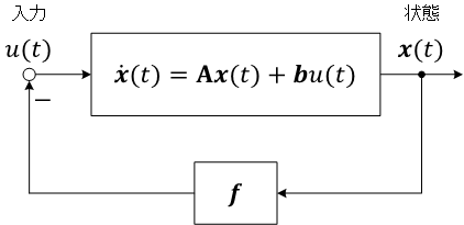閉ループ系\[ \begin{align} \dot{\boldsymbol x}(t) &= \mathbf A\boldsymbol x(t) + \boldsymbol b u(t) \\ \dot{\boldsymbol x}(t) &= \mathbf A\boldsymbol x(t) - \boldsymbol b\boldsymbol f\boldsymbol x(t) \\ \dot{\boldsymbol x}(t) &= (\mathbf A - \boldsymbol b\boldsymbol f)\boldsymbol x(t) \end{align}\]解\[ \boldsymbol x(t) = e^{(\mathbf A - \boldsymbol b\boldsymbol f)t}\boldsymbol x(0) \]

（ほかの計算方法については、教科書など）

アッカーマン(Ackerman)法（アッカーマンの極配置アルゴリズム）。Octave の control パッケージの acker() 関数を使用（具体的な計算手順については、教科書など）

システム（システムは可制御）\[ \mathbf A = \begin{bmatrix} 0 & 1 \\ -5 & -6 \end{bmatrix}, \quad \boldsymbol b = \begin{bmatrix} 0 \\ 1 \end{bmatrix} \] の固有値（極）が \( -7\pm 2j \) となるような状態フィードバックゲイン \( \boldsymbol f \) を求める

octave:1> A = [0 1; -5 -6]
A =

   0   1
  -5  -6

octave:2> b = [0; 1]
b =

   0
   1

octave:3> pkg load control
octave:4> f = acker(A, b, [-7+2i, -7-2i])
f =

   48    8

状態フィードバックゲイン\[ \boldsymbol f = \begin{pmatrix} 48 & 8 \end{pmatrix} \]

（検算）

octave:5> eig(A - b*f)
ans =

  -7.0000 + 2.0000i
  -7.0000 - 2.0000i

システムの時間応答を、初期値を \( \boldsymbol x_0 = \begin{pmatrix} 1 \\ 0\end{pmatrix} \) として、自由応答（\( u(t) = 0 \)）と状態フィードバック制御を行った場合とで比較

octave:1> type -q pole_placement.m
clear all

%% system
A = [0 1; -5 -6];
b = [0; 1];

x0 = [1; 0];

%% free response
sim_time = linspace(0, 6, 1024);

i = 1;
for t = sim_time
  x = expm(A*t)*x0;
  x_1(i) = x(1);
  x_2(i) = x(2);
  i = i + 1;
end

clf
plot(sim_time, x_1, sim_time, x_2)
grid on
xlabel("time [s]"); ylabel("state variable")

%% state feedback control
pkg load control

assert(det(ctrb(A, b)) != 0, "system is NOT controllable")
f = acker(A, b, [-7+2i, -7-2i]);

i = 1;
for t = sim_time
  x = expm((A - b*f)*t)*x0;
  x_1(i) = x(1);
  x_2(i) = x(2);
  i = i + 1;
end

hold on
plot(sim_time, x_1, sim_time, x_2)
legend("free response x_1", "free response x_2", "state feedback x_1", "state feedback x_2")
title("state feedback control")

octave:2> pole_placement

シミュレーションのためには、Octave の expm() 関数（行列指数関数）を使用して、状態遷移行列を（ラプラス変換せずに）そのまま計算。実行結果

状態変数 \( x_1 \) は位置、\( x_2 \) は速度。グラフの急峻さから、状態フィードバック制御を行ってシステムの極を \( -7\pm 2j \) へ移動するには、システムへの大きな入力が必要になることがわかる

最適制御(optimal control)

システムの応答の速さと操作量（システムへの入力）との間にはトレードオフの関係がある（最適レギュレータ問題(optimal regulator problem)）

LQR(linear quadratic regulator)

２次形式(quadratic form)の評価関数(evaluation function)（損失関数(loss function)、コスト関数(cost function)）を用いて、状態フィードバックゲインを求める

評価関数\[ J = \frac{1}{2}\int_0^\infty\left\{ \boldsymbol x^{\mathsf T}(t)\mathbf Q\boldsymbol x(t) + \boldsymbol u^{\mathsf T}(t)\mathbf R\boldsymbol u(t) \right\}\, dt \]（\( J \) はスカラー）

ここで、\( \mathbf Q,\, \mathbf R \) は重み係数行列。\( \mathbf Q \) は \( n\times n \) の半正定対称行列、\( \mathbf R \) は \( p\times p \) の正定対称行列

（\( J \) を最小にする）最適制御は\[ \boldsymbol u(t) = -\mathbf F\boldsymbol x(t) = -\mathbf R^{-1}\mathbf B^{\mathsf T}\mathbf P\boldsymbol x(t) \]で与えられる。状態フィードバックゲインは\[ \begin{align} -\mathbf F\boldsymbol x(t) &= -\mathbf R^{-1}\mathbf B^{\mathsf T}\mathbf P\boldsymbol x(t) \\ \mathbf F &= \mathbf R^{-1}\mathbf B^{\mathsf T}\mathbf P \end{align} \]となる

\( \mathbf P \) は（\( \mathbf P \) 以外はすべて既知）、リカッチ代数方程式(algebraic Riccati equation)\[ \mathbf A^\mathsf T\mathbf P + \mathbf P\mathbf A + \mathbf Q - \mathbf P\mathbf B\mathbf R^{-1}\mathbf B^\mathsf T\mathbf P = \mathbf 0 \]の解（唯一の正定対称解）

\( \mathbf P \) は \( n\times n \) の正定対称行列になる（式の導出、解き方については、教科書など）

（正定行列、半正定行列については、線形代数）

Octave の control パッケージの lqr() 関数を使用。重みを変更しながらシミュレーション

octave:1> type -q sim_lqr.m
clear all

%% system
A = [0 1; -5 -6]; B = [0; 1];

pkg load control
assert(det(ctrb(A, B)) != 0, "system is NOT controllable")
assert((det(ctrb(A, B)) != 0) == (rank(ctrb(A, B)) == size(A)(1)))

x0 = [1; 0];

%% LQR
sim_time = linspace(0, 6, 1024);

Q = [1 0; 0 1]; R = 1;

clf
for weight = [1, 10, 100, 1000]
  Q(1,1) = weight;
  [G, X, L] = lqr(A, B, Q, R);

  i = 1;
  for t = sim_time
    x = expm((A - B*G)*t)*x0;
    x_1(i) = x(1);
    x_2(i) = x(2);
    i = i + 1;
  end
  plot(sim_time, x_1, sim_time, x_2)
  hold on
end
grid on
legend("x_1", "x_2"); xlabel("time [s]"); ylabel("state")
title("Q_1_1 = 1, 10, 100, 1000")

pause()

%% LQR
Q = [1 0; 0 1]; R = 1;

clf
for weight = [1, 10, 100, 1000]
  Q(2,2) = weight;
  [G, X, L] = lqr(A, B, Q, R);

  i = 1;
  for t = sim_time
    x = expm((A - B*G)*t)*x0;
    x_1(i) = x(1);
    x_2(i) = x(2);
    i = i + 1;
  end
  plot(sim_time, x_1, sim_time, x_2)
  hold on
end
grid on
legend("x_1", "x_2"); xlabel("time [s]"); ylabel("state")
title("Q_2_2 = 1, 10, 100, 1000")

pause()

%% LQR
Q = [1 0; 0 1]; R = 1;

clf
for weight = [1, 0.1, 0.01, 0.001]
  R = weight;
  [G, X, L] = lqr(A, B, Q, R);

  i = 1;
  for t = sim_time
    x = expm((A - B*G)*t)*x0;
    x_1(i) = x(1);
    x_2(i) = x(2);
    i = i + 1;
  end
  plot(sim_time, x_1, sim_time, x_2)
  hold on
end
grid on
legend("x_1", "x_2"); xlabel("time [s]"); ylabel("state")
title("R = 1, 0.1, 0.01, 0.001")

octave:2> sim_lqr

実行結果

重み \( Q_{11} = \{ 1, 10, 100, 1000 \} \)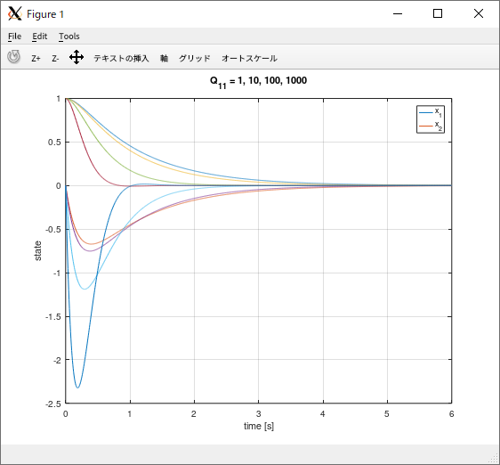
重み \( Q_{22} = \{ 1, 10, 100, 1000 \} \)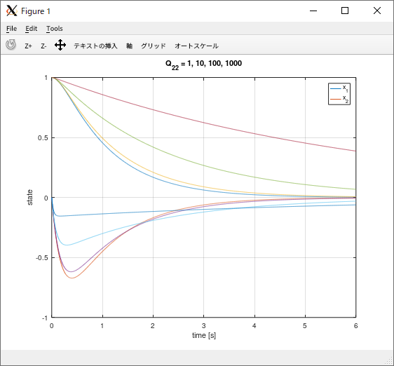
重み \( R = \{ 1, 0.1, 0.01, 0.001 \} \)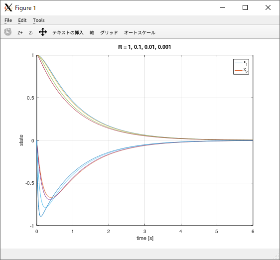

\( \mathbf Q \) と \( \mathbf R \) は設計者が決定して与える。通常、（対角成分がすべて正の値の）対角行列を使うことが多い

サーボシステム(servo system)

（レギュレーターでは、定常的な外乱がある場合に、状態変数が 0 にならない）

外乱を抑制し、かつ、目標値 \( r(t) \) に出力 \( y(t)\) を定常偏差(steady state error)なく追従させる（サーボ制御(servo control)）

（図で、\( \boxed{ \frac{1}{s} } \) は積分器。\( \boldsymbol c \) と \( \boldsymbol f \) は行ベクトル）

（内部モデル原理(internal model principle)について → 教科書など）

状態フィードバック制御 + 積分制御（I 制御）\[ \left\{ \begin{align} & \dot{\boldsymbol x}(t) = \mathbf A\boldsymbol x(t) + \boldsymbol b u(t) + \boldsymbol v(t) \\ & y(t) = \boldsymbol c\boldsymbol x(t) \end{align} \right. \]\[ \left\{ \begin{align} & u(t) = -\boldsymbol f\boldsymbol x(t) + k z(t) \\ & \dot z(t) = e(t) = r(t) - y(t) \end{align} \right. \]

\( \boldsymbol v(t) \) は外乱。\( k \) は積分ゲイン

拡大系

状態方程式\[ \begin{bmatrix} \dot{\boldsymbol x}(t) \\ \dot z(t) \end{bmatrix} = \begin{bmatrix} \mathbf A & 0 \\ -\boldsymbol c & 0 \end{bmatrix}\begin{bmatrix} \boldsymbol x(t) \\ z(t) \end{bmatrix} + \begin{bmatrix} \boldsymbol b \\ 0 \end{bmatrix}u(t) + \begin{bmatrix} \boldsymbol v(t) \\ r(t) \end{bmatrix} \]

\( \begin{bmatrix} \boldsymbol x(t) \\ z(t) \end{bmatrix} \) は拡大系の状態変数

拡大系に対する、状態フィードバック制御\[ u(t) = -\begin{bmatrix} \boldsymbol f & -k \end{bmatrix}\begin{bmatrix} \boldsymbol x(t) \\ z(t) \end{bmatrix} \]

拡大系が可制御であると仮定して、状態フィードバック制御\[ u(t) = -\begin{bmatrix} \boldsymbol f^* & -k^* \end{bmatrix}\begin{bmatrix} \boldsymbol x(t) \\ z(t) \end{bmatrix} \]を考える。\( \boldsymbol f^* \) と \( k^* \) はシステムが漸近安定になるように適切に決定されたフィードバックゲイン

閉ループ系\[ \begin{align} \begin{bmatrix} \dot{\boldsymbol x}(t) \\ \dot z(t) \end{bmatrix} &= \begin{bmatrix} \mathbf A & 0 \\ -\boldsymbol c & 0 \end{bmatrix}\begin{bmatrix} \boldsymbol x(t) \\ z(t) \end{bmatrix} + \begin{bmatrix} \boldsymbol b \\ 0 \end{bmatrix}\left\{ -\begin{bmatrix} \boldsymbol f^* & -k^* \end{bmatrix}\begin{bmatrix} \boldsymbol x(t) \\ z(t) \end{bmatrix} \right\} + \begin{bmatrix} \boldsymbol v(t) \\ r(t) \end{bmatrix} \\ &= \begin{bmatrix} \mathbf A & 0 \\ -\boldsymbol c & 0 \end{bmatrix}\begin{bmatrix} \boldsymbol x(t) \\ z(t) \end{bmatrix} + \begin{bmatrix} \boldsymbol b \\ 0 \end{bmatrix}\begin{bmatrix} -\boldsymbol f^* & k^* \end{bmatrix}\begin{bmatrix} \boldsymbol x(t) \\ z(t) \end{bmatrix} + \begin{bmatrix} \boldsymbol v(t) \\ r(t) \end{bmatrix} \\ &= \begin{bmatrix} \mathbf A & 0 \\ -\boldsymbol c & 0 \end{bmatrix}\begin{bmatrix} \boldsymbol x(t) \\ z(t) \end{bmatrix} + \begin{bmatrix} -\boldsymbol b\boldsymbol f^* & \boldsymbol b k^* \\ 0 & 0 \end{bmatrix}\begin{bmatrix} \boldsymbol x(t) \\ z(t) \end{bmatrix} + \begin{bmatrix} \boldsymbol v(t) \\ r(t) \end{bmatrix} \\ &= \begin{bmatrix} \mathbf A - \boldsymbol b\boldsymbol f^* & \boldsymbol b k^* \\ -\boldsymbol c & 0 \end{bmatrix}\begin{bmatrix} \boldsymbol x(t) \\ z(t) \end{bmatrix} + \begin{bmatrix} \boldsymbol v(t) \\ r(t) \end{bmatrix} \end{align} \]

\( \boldsymbol v(t) \) と \( r(t) \) はステップ信号とする

システムは内部安定(internal stability)。t → ∞ で\[ \lim_{t \to \infty}\begin{bmatrix} \boldsymbol x(t) \\ z(t) \end{bmatrix} = \begin{bmatrix} \boldsymbol x(\infty) \\ z(\infty) \end{bmatrix} \]拡大系の状態（\( \boldsymbol x(\infty) \) と \( z(\infty) \)）は一定値に収束する。よって、\[ \lim_{t \to \infty}\begin{bmatrix} \dot{\boldsymbol x}(t) \\ \dot z(t) \end{bmatrix} = \begin{bmatrix} \boldsymbol 0 \\ 0 \end{bmatrix} \]

t → ∞ で\[ \begin{bmatrix} \boldsymbol 0 \\ 0 \end{bmatrix} = \begin{bmatrix} \mathbf A - \boldsymbol b\boldsymbol f^* & \boldsymbol b k^* \\ -\boldsymbol c & 0 \end{bmatrix}\begin{bmatrix} \boldsymbol x(\infty) \\ z(\infty) \end{bmatrix} + \begin{bmatrix} \boldsymbol v_0 \\ r_0 \end{bmatrix} \]が成り立つ

（行列 \( \begin{bmatrix} \mathbf A - \boldsymbol b\boldsymbol f^* & \boldsymbol b k^* \\ -\boldsymbol c & 0 \end{bmatrix} \) は安定なので（そのように \( \boldsymbol f^* \) と \( k^* \) を決定している）、すべての固有値の実部は負（≠ 0）のため逆行列を持つ \( \boxed{ |\mathbf A| = \lambda_1\lambda_2\cdots\lambda_n } \)）\[ \begin{align} \begin{bmatrix} \boldsymbol 0 \\ 0 \end{bmatrix} &= \begin{bmatrix} \mathbf A - \boldsymbol b\boldsymbol f^* & \boldsymbol b k^* \\ -\boldsymbol c & 0 \end{bmatrix}\begin{bmatrix} \boldsymbol x(\infty) \\ z(\infty) \end{bmatrix} + \begin{bmatrix} \boldsymbol v_0 \\ r_0 \end{bmatrix} \\ -\begin{bmatrix} \mathbf A - \boldsymbol b\boldsymbol f^* & \boldsymbol b k^* \\ -\boldsymbol c & 0 \end{bmatrix}\begin{bmatrix} \boldsymbol x(\infty) \\ z(\infty) \end{bmatrix} &= \begin{bmatrix} \boldsymbol v_0 \\ r_0 \end{bmatrix} \\ \begin{bmatrix} \boldsymbol x(\infty) \\ z(\infty) \end{bmatrix} &= -\begin{bmatrix} \mathbf A - \boldsymbol b\boldsymbol f^* & \boldsymbol b k^* \\ -\boldsymbol c & 0 \end{bmatrix}^{-1}\begin{bmatrix} \boldsymbol v_0 \\ r_0 \end{bmatrix} \end{align} \]

拡大系の偏差\[ \begin{align} e(\infty) &= r_0 - y(\infty) \\ &= r_0 - \bar{\boldsymbol c}\bar{\boldsymbol x}(\infty) \\ &= r_0 - \begin{bmatrix} \boldsymbol c & 0 \end{bmatrix}\begin{bmatrix} \boldsymbol x(\infty) \\ z(\infty) \end{bmatrix} \\ &= r_0 - \begin{bmatrix} \boldsymbol c & 0 \end{bmatrix}\left\{ -\begin{bmatrix} \mathbf A - \boldsymbol b\boldsymbol f^* & \boldsymbol b k^* \\ -\boldsymbol c & 0 \end{bmatrix}^{-1}\begin{bmatrix} \boldsymbol v_0 \\ r_0 \end{bmatrix} \right\} \\ &= r_0 + \begin{bmatrix} \boldsymbol c & 0 \end{bmatrix}\begin{bmatrix} \mathbf A - \boldsymbol b\boldsymbol f^* & \boldsymbol b k^* \\ -\boldsymbol c & 0 \end{bmatrix}^{-1}\begin{bmatrix} \boldsymbol v_0 \\ r_0 \end{bmatrix} \\ &= r_0 + \left\{ \begin{bmatrix} 0 & -1 \end{bmatrix}\begin{bmatrix} \mathbf A - \boldsymbol b\boldsymbol f^* & \boldsymbol b k^* \\ -\boldsymbol c & 0 \end{bmatrix} \right\}\begin{bmatrix} \mathbf A - \boldsymbol b\boldsymbol f^* & \boldsymbol b k^* \\ -\boldsymbol c & 0 \end{bmatrix}^{-1}\begin{bmatrix} \boldsymbol v_0 \\ r_0 \end{bmatrix} \\ &= r_0 + \begin{bmatrix} 0 & -1 \end{bmatrix}\begin{bmatrix} \mathbf A - \boldsymbol b\boldsymbol f^* & \boldsymbol b k^* \\ -\boldsymbol c & 0 \end{bmatrix}\begin{bmatrix} \mathbf A - \boldsymbol b\boldsymbol f^* & \boldsymbol b k^* \\ -\boldsymbol c & 0 \end{bmatrix}^{-1}\begin{bmatrix} \boldsymbol v_0 \\ r_0 \end{bmatrix} \\ &= r_0 + \begin{bmatrix} 0 & -1 \end{bmatrix}\begin{bmatrix} \boldsymbol v_0 \\ r_0 \end{bmatrix} \\ &= r_0 -r_0 \\ &= 0 \end{align} \]（式変形のテクニック \( \boxed{ \begin{bmatrix} 0 & -1 \end{bmatrix}\begin{bmatrix} \mathbf A - \boldsymbol b\boldsymbol f^* & \boldsymbol b k^* \\ -\boldsymbol c & 0 \end{bmatrix} = \begin{bmatrix} \boldsymbol c & 0 \end{bmatrix} } \)）

偏差 \(e(\infty) = 0 \) となるので \( y(\infty) = r_0 \)（∴ サーボ制御を達成）

ここで\[ \begin{gather} \bar{\boldsymbol x}(t) = \begin{bmatrix} \boldsymbol x(t) \\ z(t) \end{bmatrix}, \quad \bar{\mathbf A} = \begin{bmatrix} \mathbf A & 0 \\ -\boldsymbol c & 0 \end{bmatrix}, \quad \bar{\boldsymbol b} = \begin{bmatrix} \boldsymbol b \\ 0 \end{bmatrix}, \quad \bar{\boldsymbol f} = \begin{bmatrix} \boldsymbol f & -k \end{bmatrix} \end{gather} \]と置きなおして、行列の形で再度式を整理

拡大系の状態フィードバック制御\[ \left\{ \begin{align} & \dot{\bar{\boldsymbol x}}(t) = \bar{\mathbf A}\bar{\boldsymbol x}(t) + \bar{\boldsymbol b}u(t) + \begin{bmatrix} \boldsymbol v(t) \\ r(t) \end{bmatrix} \\ & u(t) = -\bar{\boldsymbol f}\bar{\boldsymbol x}(t) \end{align} \right. \]閉ループ系 \[ \dot{\bar{\boldsymbol x}}(t) = (\bar{\mathbf A} - \bar{\boldsymbol b}\bar{\boldsymbol f})\bar{\boldsymbol x}(t) + \begin{bmatrix} \boldsymbol v(t) \\ r(t) \end{bmatrix} \]

サーボ制御の設計

システム\[ \left\{ \begin{align} & \dot{\boldsymbol x}(t) = \begin{pmatrix} 0 & 1 \\ -5 & -6 \end{pmatrix} + \begin{pmatrix} 0 \\ 1 \end{pmatrix}u(t) + \boldsymbol v(t) \\ & y(t) = \begin{pmatrix} 1 & 0 \end{pmatrix}\boldsymbol x(t) \end{align} \right. \]

\( \boldsymbol v(t) = \boldsymbol 0 \) として、拡大系を構成\[ \begin{bmatrix} \dot x_1(t) \\ \dot x_2(t) \\ \dot z(t) \end{bmatrix} = \begin{pmatrix} 0 & 1 & 0 \\ -5 & -6 & 0 \\ -1 & 0 & 0 \end{pmatrix}\begin{bmatrix} x_1(t) \\ x_2(t) \\ z(t) \end{bmatrix} + \begin{pmatrix} 0 \\ 1 \\ 0 \end{pmatrix}u(t) \]

変数を置きなおして\[ \begin{gather} \dot{\bar{\boldsymbol x}}(t) = \bar{\mathbf A}\bar{\boldsymbol x}(t) + \bar{\boldsymbol b}u(t) \\ \bar{\mathbf A} = \begin{pmatrix} 0 & 1 & 0 \\ -5 & -6 & 0 \\ -1 & 0 & 0 \end{pmatrix}, \quad \bar{\boldsymbol b} = \begin{pmatrix} 0 \\ 1 \\ 0 \end{pmatrix} \end{gather} \]

拡大系の状態フィードバック制御\[ u(t) = -\begin{pmatrix} f_1 & f_2 & -k \end{pmatrix}\bar{\boldsymbol x}(t) \]

閉ループ系の固有値（極）を -3 の３重根とする、状態フィードバックゲイン

octave:1> Abar = [0 1 0; -5 -6 0; -1 0 0]
Abar =

   0   1   0
  -5  -6   0
  -1   0   0

octave:2> bbar = [0; 1; 0]
bbar =

   0
   1
   0

octave:3> pkg load control
octave:4> det(ctrb(Abar, bbar))
ans =  1
octave:5> fbar = acker(Abar, bbar, [-3, -3, -3])
fbar =

   22    3  -27

octave:6> fbar = place(Abar, bbar, [-3, -3, -3])
fbar =

   22.0000    3.0000  -27.0000

（※acker() 関数、place() 関数については、Octave の control パッケージのドキュメントを参照）

状態フィードバックゲイン\[ \begin{gather} \bar{\boldsymbol f} = \begin{bmatrix} f_1 & f_2 & -k \end{bmatrix} = \begin{pmatrix} 22 & 3 & -27 \end{pmatrix} \\ \boldsymbol f = \begin{pmatrix} 22 & 3 \end{pmatrix}, \quad k = 27 \end{gather}\]

ステップ状の目標値 \( r(t) = \begin{cases} r_0 & (t \ge 0) \\ 0 & (t \lt 0) \end{cases} \) と外乱 \( \boldsymbol v(t) = \begin{cases} \boldsymbol v_0 & (t \ge 0) \\ 0 & (t \lt 0) \end{cases} \) （定値外乱）に対して、定常偏差が残らないことを確認

閉ループ系\[ \begin{align} \dot{\bar{\boldsymbol x}}(t) &= (\bar{\mathbf A} - \bar{\boldsymbol b}\bar{\boldsymbol f})\bar{\boldsymbol x}(t) + \begin{bmatrix} \boldsymbol v(t) \\ r(t) \end{bmatrix} \\ &= \left\{ \begin{pmatrix} 0 & 1 & 0 \\ -5 & -6 & 0 \\ -1 & 0 & 0 \end{pmatrix} - \begin{pmatrix} 0 \\ 1 \\ 0 \end{pmatrix}\begin{pmatrix} 22 & 3 & -27 \end{pmatrix} \right\}\bar{\boldsymbol x}(t) + \begin{bmatrix} \boldsymbol v(t) \\ r(t) \end{bmatrix} \\ &= \left\{ \begin{pmatrix} 0 & 1 & 0 \\ -5 & -6 & 0 \\ -1 & 0 & 0 \end{pmatrix} - \begin{pmatrix} 0 & 0 & 0 \\ 22 & 3 & -27 \\ 0 & 0 & 0 \end{pmatrix} \right\}\bar{\boldsymbol x}(t) + \begin{bmatrix} \boldsymbol v(t) \\ r(t) \end{bmatrix} \\ &= \begin{pmatrix} 0 & 1 & 0 \\ -27 & -9 & 27 \\ -1 & 0 & 0 \end{pmatrix}\bar{\boldsymbol x}(t) + \begin{bmatrix} \boldsymbol v(t) \\ r(t) \end{bmatrix} \end{align} \]

（上記と同様に）\( \dot{\bar{\boldsymbol x}}(\infty) = \boldsymbol 0 \)\[ \begin{align} \dot{\bar{\boldsymbol x}}(\infty) &= \begin{pmatrix} 0 & 1 & 0 \\ -27 & -9 & 27 \\ -1 & 0 & 0 \end{pmatrix}\bar{\boldsymbol x}(\infty) + \begin{bmatrix} \boldsymbol v(\infty) \\ r(\infty) \end{bmatrix} \\ \begin{bmatrix} 0 \\ 0 \\ 0 \end{bmatrix} &= \begin{pmatrix} 0 & 1 & 0 \\ -27 & -9 & 27 \\ -1 & 0 & 0 \end{pmatrix}\begin{bmatrix} x_1(\infty) \\ x_2(\infty) \\ z(\infty) \end{bmatrix} + \begin{bmatrix} v_1(\infty) \\ v_2(\infty) \\ r(\infty) \end{bmatrix} \\ -\begin{pmatrix} 0 & 1 & 0 \\ -27 & -9 & 27 \\ -1 & 0 & 0 \end{pmatrix}\begin{bmatrix} x_1(\infty) \\ x_2(\infty) \\ z(\infty) \end{bmatrix} &= \begin{bmatrix} v_1(\infty) \\ v_2(\infty) \\ r(\infty) \end{bmatrix} \\ \begin{bmatrix} x_1(\infty) \\ x_2(\infty) \\ z(\infty) \end{bmatrix} &= -\begin{pmatrix} 0 & 1 & 0 \\ -27 & -9 & 27 \\ -1 & 0 & 0 \end{pmatrix}^{-1}\begin{bmatrix} v_1(\infty) \\ v_2(\infty) \\ r(\infty) \end{bmatrix} \\ \begin{bmatrix} x_1(\infty) \\ x_2(\infty) \\ z(\infty) \end{bmatrix} &= -\begin{pmatrix} 0 & 0 & -1 \\ 1 & 0 & 0 \\ \frac{1}{3} & \frac{1}{27} & -1 \end{pmatrix}\begin{bmatrix} v_1(\infty) \\ v_2(\infty) \\ r(\infty) \end{bmatrix} \\ \begin{bmatrix} x_1(\infty) \\ x_2(\infty) \\ z(\infty) \end{bmatrix} &= \begin{pmatrix} 0 & 0 & 1 \\ -1 & 0 & 0 \\ -\frac{1}{3} & -\frac{1}{27} & 1 \end{pmatrix}\begin{bmatrix} v_1(\infty) \\ v_2(\infty) \\ r(\infty) \end{bmatrix} \\ \begin{bmatrix} x_1(\infty) \\ x_2(\infty) \\ z(\infty) \end{bmatrix} &= \begin{bmatrix} r(\infty) \\ -v_1(\infty) \\ -\frac{1}{3}v_1(\infty) - \frac{1}{27}v_2(\infty) + r(\infty) \end{bmatrix} \end{align} \]

（状態変数 \( x_1 \) は位置）\[ \therefore\, x_1(\infty) = r(\infty) \]

オブザーバ(observer)

（直接観測することのできない、）状態変数 \( \boldsymbol x(t) \) を推定する（状態観測器）

同一次元オブザーバ(identity observer (full order observer))

（制御対象）システム\[ \left\{ \begin{align} & \dot{\boldsymbol x}(t) = \mathbf A\boldsymbol x(t) + \mathbf B\boldsymbol u(t) \\ & \boldsymbol y(t) = \mathbf C\boldsymbol x(t) \end{align} \right. \]

システムが可観測であれば、直接観測できない状態変数 \( \boldsymbol x(t) \) を推定できる。推定された状態変数を \( \hat{\boldsymbol x}(t) \) （\( \boldsymbol x(t) \) と \( \hat{\boldsymbol x}(t) \) は、同じ次元のベクトル）

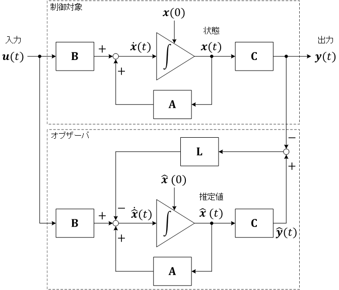
図で、\( \mathbf L \) はオブザーバゲイン。\( \boldsymbol x(0) \) と \( \hat{\boldsymbol x}(0) \) は状態変数の初期値

オブザーバ\[ \left\{ \begin{align} & \dot{\hat{\boldsymbol x}}(t) = \mathbf A\hat{\boldsymbol x}(t) + \mathbf B\boldsymbol u(t) - \mathbf L\left( \hat{\boldsymbol y}(t) - \boldsymbol y(t) \right) \\ & \hat{\boldsymbol y}(t) = \mathbf C\hat{\boldsymbol x}(t) \end{align} \right. \]

\( \hat{\boldsymbol x}(t) \) と \( \boldsymbol x(t) \) が一致することを確認\[ \boldsymbol \eta(t) = \hat{\boldsymbol x}(t) - \boldsymbol x(t) \]と置く

（両辺を微分。オブザーバの式から制御対象のシステムの式を引く）\[ \begin{align} \boldsymbol \eta(t) &= \hat{\boldsymbol x}(t) - \boldsymbol x(t) \\ \dot{\boldsymbol \eta}(t) &= \dot{\hat{\boldsymbol x}}(t) - \dot{\boldsymbol x}(t) \\ &= \mathbf A\hat{\boldsymbol x}(t) + \mathbf B\boldsymbol u(t) - \mathbf L\left( \hat{\boldsymbol y}(t) - \boldsymbol y(t) \right) - \mathbf A\boldsymbol x(t) - \mathbf B\boldsymbol u(t) \\ &= \mathbf A\hat{\boldsymbol x}(t) + \mathbf B\boldsymbol u(t) - \mathbf L\left( \mathbf C\hat{\boldsymbol x}(t) - \mathbf C\boldsymbol x(t) \right) - \mathbf A\boldsymbol x(t) - \mathbf B\boldsymbol u(t) \\ &= \mathbf A\hat{\boldsymbol x}(t) - \mathbf A\boldsymbol x(t) - \mathbf L\left( \mathbf C\hat{\boldsymbol x}(t) - \mathbf C\boldsymbol x(t) \right) \\ &= \mathbf A\left( \hat{\boldsymbol x}(t) - \boldsymbol x(t) \right) - \mathbf L\mathbf C\left( \hat{\boldsymbol x}(t) - \boldsymbol x(t) \right) \\ &= \mathbf A\boldsymbol \eta(t) - \mathbf L\mathbf C\boldsymbol \eta(t) \\ &= (\mathbf A - \mathbf L\mathbf C)\boldsymbol \eta(t) \end{align} \]

推定誤差\[ \dot{\boldsymbol \eta}(t) = (\mathbf A - \mathbf L\mathbf C)\boldsymbol \eta(t) \]

（cf. 状態方程式の解）自由応答\[ \begin{gather} \dot{\boldsymbol x}(t) = \mathbf A\boldsymbol x(t) \\ \boldsymbol x(t) = e^{\mathbf At}\boldsymbol x(0) \end{gather} \]

同様に解く\[ \boldsymbol \eta(t) = e^{(\mathbf A - \mathbf L\mathbf C)t}\boldsymbol \eta(0) \]となる

（ここで\[ \boldsymbol \eta(0) = \hat{\boldsymbol x}(0) - \boldsymbol x(0) \]で \( \boldsymbol \eta(0) \) は未知）

もし、漸近安定（行列 \( \boxed{ (\mathbf A - \mathbf L\mathbf C) } \) のすべての固有値の実部が負）ならば\[ \lim_{t \to \infty}\boldsymbol\eta(t) = \boldsymbol 0 \]となり\[ \therefore\, \hat{\boldsymbol x}(\infty) = \boldsymbol x(\infty) \]

（行列 \( \boxed{ (\mathbf A - \mathbf L\mathbf C) } \) の固有値をオブザーバの極）

オブザーバの設計

システム\[ \left\{ \begin{align} & \dot{\boldsymbol x}(t) = \begin{pmatrix} 0 & 1 \\ -5 & -6 \end{pmatrix} + \begin{pmatrix} 0 \\ 1 \end{pmatrix}u(t) \\ & y(t) = \begin{pmatrix} 1 & 0 \end{pmatrix}\boldsymbol x(t) \end{align} \right. \]

オブザーバの極（\( \mathbf A - \mathbf L\mathbf C \) の固有値）を \( -7,\, -8 \) に配置

（可制御性と可観測性の双対性(duality)（双対なシステム(dual system)）について → 教科書など）

\( \mathbf A^\mathsf T \rightarrow \mathbf A^*,\, \mathbf C^\mathsf T \rightarrow \mathbf B^* \) と置き換え、状態フィードバック制御による極配置と同様に解く

octave:1> A = [0 1; -5 -6]
A =

   0   1
  -5  -6

octave:2> B = [0; 1]
B =

   0
   1

octave:3> C = [1 0]
C =

   1   0

octave:4> pkg load control
octave:5> det(obsv(A, C))
ans =  1
octave:6> Aast = A'
Aast =

   0  -5
   1  -6

octave:7> Bast = C'
Bast =

   1
   0

octave:8> F = acker(Aast, Bast, [-7, -8])
F =

   9  -3

octave:9> place(Aast, Bast, [-7, -8])
ans =

   9.0000  -3.0000

octave:10> L = F'
L =

   9
  -3

オブザーバゲイン\[ \mathbf L = \begin{pmatrix} 9 \\ -3 \end{pmatrix} \]

（制御対象のシステムの極に対して、オブザーバの極を適切に配置する → 教科書など）

併合系

（オブザーバゲイン \( \mathbf L \) と状態フィードバックゲイン \( \mathbf F \) とは、独立に設計できる → 教科書など）

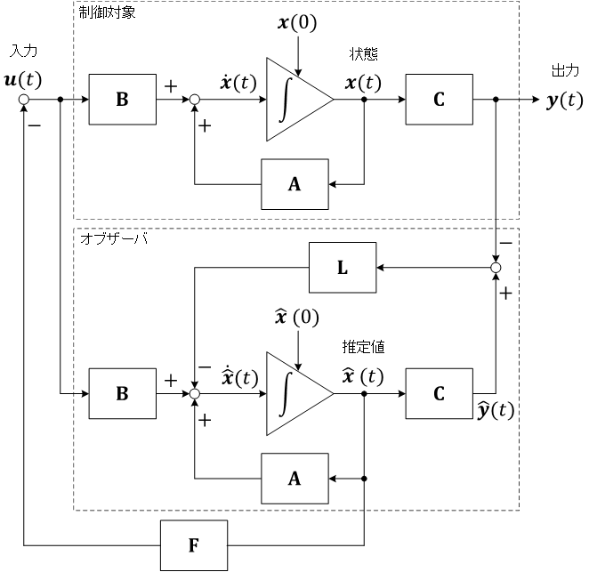
オブザーバを用いた状態フィードバック制御\[ \left\{ \begin{align} & \boldsymbol u(t) = -\mathbf F\hat{\boldsymbol x}(t) \\ & \dot{\hat{\boldsymbol x}}(t) = \left( \mathbf A - \mathbf L\mathbf C \right)\hat{\boldsymbol x}(t) + \mathbf L\boldsymbol y(t) + \mathbf B\boldsymbol u(t) \end{align} \right. \]

（オブザーバの式）\[ \boxed{ \begin{align} \dot{\hat{\boldsymbol x}}(t) &= \mathbf A\hat{\boldsymbol x}(t) + \mathbf B\boldsymbol u(t) - \mathbf L\left( \hat{\boldsymbol y}(t) - \boldsymbol y(t) \right) \\ &= \mathbf A\hat{\boldsymbol x}(t) + \mathbf B\boldsymbol u(t) - \mathbf L\left( \mathbf C\hat{\boldsymbol x}(t) - \boldsymbol y(t) \right) \\ &= \mathbf A\hat{\boldsymbol x}(t) + \mathbf B\boldsymbol u(t) - \mathbf L\mathbf C\hat{\boldsymbol x}(t) + \mathbf L\boldsymbol y(t) \\ &= \left\{ \mathbf A\hat{\boldsymbol x}(t) - \mathbf L\mathbf C\hat{\boldsymbol x}(t) \right\} + \mathbf B\boldsymbol u(t) + \mathbf L\boldsymbol y(t) \\ &= \left( \mathbf A - \mathbf L\mathbf C \right)\hat{\boldsymbol x}(t) + \mathbf B\boldsymbol u(t) + \mathbf L\boldsymbol y(t) \end{align} }\]

オブザーバと状態フィードバック制御の併合系

（制御対象の状態方程式\[ \dot{\boldsymbol x}(t) = \mathbf A\boldsymbol x(t) - \mathbf B\mathbf F\hat{\boldsymbol x}(t) \]と、オブザーバの式\[ \boxed{ \begin{align} \dot{\hat{\boldsymbol x}}(t) &= \left( \mathbf A - \mathbf L\mathbf C \right)\hat{\boldsymbol x}(t) + \mathbf B\boldsymbol u(t) + \mathbf L\boldsymbol y(t) \\ &= \left( \mathbf A - \mathbf L\mathbf C \right)\hat{\boldsymbol x}(t) - \mathbf B\mathbf F\hat{\boldsymbol x}(t) + \mathbf L\mathbf C\boldsymbol x(t) \\ &= \left( \mathbf A - \mathbf L\mathbf C - \mathbf B\mathbf F \right)\hat{\boldsymbol x}(t) + \mathbf L\mathbf C\boldsymbol x(t) \end{align} } \]とを\[ \left\{ \begin{align} & \dot{\boldsymbol x}(t) = \mathbf A\boldsymbol x(t) - \mathbf B\mathbf F\hat{\boldsymbol x}(t) \\ & \dot{\hat{\boldsymbol x}}(t) = \mathbf L\mathbf C\boldsymbol x(t) + \left( \mathbf A - \mathbf L\mathbf C - \mathbf B\mathbf F \right)\hat{\boldsymbol x}(t) \end{align} \right. \]行列の形で再度式を整理）\[ \begin{bmatrix} \dot{\boldsymbol x}(t) \\ \dot{\hat{\boldsymbol x}}(t) \end{bmatrix} = \begin{pmatrix} \mathbf A & -\mathbf B\mathbf F \\ \mathbf L\mathbf C & \mathbf A - \mathbf B\mathbf F - \mathbf L\mathbf C \end{pmatrix}\begin{bmatrix} \boldsymbol x(t) \\ \hat{\boldsymbol x}(t) \end{bmatrix}\]

併合系の固有値（システムの極）が、状態フィードバック制御の閉ループ系の固有値とオブザーバの固有値からなることを確認

（上記の計算結果）

• 状態フィードバック制御

• 固有値（閉ループシステムの極） : \( -7\pm 2j \)

• 状態フィードバックゲイン : \( \mathbf F = \begin{pmatrix} 48 & 8 \end{pmatrix} \)
• オブザーバ
• 固有値（オブザーバの極） : \( -7,\, -8 \)
• オブザーバゲイン : \( \mathbf L = \begin{pmatrix} 9 \\ -3 \end{pmatrix} \)

octave:1> A = [0 1; -5 -6]
A =

   0   1
  -5  -6

octave:2> B = [0; 1]
B =

   0
   1

octave:3> C = [1 0]
C =

   1   0

octave:4> F = [48 8]
F =

   48    8

octave:5> L = [9; -3]
L =

   9
  -3

octave:6> eig([A -B*F; L*C A-B*F-L*C])
ans =

  -7.0000 + 2.0000i
  -7.0000 - 2.0000i
  -8.0000 + 0.0000i
  -7.0000 + 0.0000i

オブザーバを用いた状態フィードバック制御の設計

併合系の設計。状態フィードバック制御の設計とオブザーバの設計とは、独立して設計することができる（詳細や証明は、教科書など）

• 状態フィードバックゲイン \( \mathbf F \) は、状態変数 \( \boldsymbol x(t) \) がすべて観測できるとして設計

• オブザーバが推定した状態変数 \( \hat{\boldsymbol x}(t) \) を用いて状態フィードバック制御を行う

オイラー(Euler)>法

数値解法による、状態方程式の解（数値積分）

システム\[ \begin{gather} \dot{\boldsymbol x}(t) = \mathbf A\boldsymbol x(t) + \mathbf Bu(t) \\ \mathbf A = \begin{bmatrix} 0 & 1 \\ -5 & -6 \end{bmatrix},\quad \mathbf B = \begin{bmatrix} 0 \\ 1 \end{bmatrix} \end{gather} \]の時間応答

状態変数の初期値は \( \boldsymbol x_0 = \begin{bmatrix} 0 \\ 0 \end{bmatrix} \)、入力 \( u(t) \) は矩形波（ここでは、状態変数 \( \boldsymbol x(t) \) は直接観測できるとする）

プログラム

octave:1> type -q euler.m
clear all

A = [0 1; -5 -6];
B = [0; 1];

dt = 0.001;
sim_time = 0:dt:6;

i = 1;
for t = sim_time
  if mod(t, 1) > 0.5 
    u = 0;
  else
    u = 1;
  end
  if t == 0
    x = [0; 0]; % x0
  else
    dx = A*x + B*u;
    x = x + dx*dt;
  end
  x_1(i) = x(1);
  x_2(i) = x(2);
  i = i + 1;
end

clf
plot(sim_time, x_1)
hold
plot(sim_time, x_2)
grid on
legend("x_1", "x_2")
xlabel("time [s]"); ylabel("state vector")
title("time response")
print("fig_euler_octave.png", "-dpng")

octave:2> euler

In [1]: %cat euler.py
import numpy as np

A = np.array([[0, 1], [-5, -6]])
B = np.array([[0], [1]])

dt = 0.001
sim_time = np.arange(0, 6, dt)

x_1 = []; x_2 = []
for t in sim_time:
    u = 0 if (t%1) > 0.5 else 1
    if t == 0:
        x = np.array([[0], [0]]) # x0
    else:
        dx = A@x + B*u
        x = x + dx*dt
    x_1.append(x[0])
    x_2.append(x[1])

import matplotlib.pyplot as plt

plt.clf(); plt.grid()
plt.plot(sim_time, x_1, label=r'$ x_1 $')
plt.plot(sim_time, x_2, label=r'$ x_2 $')
plt.legend(loc='best')
plt.xlabel('time [s]'); plt.ylabel('state vector')
plt.title('time response')
plt.savefig('fig_euler.png')

In [2]: %run euler.py

解（シミュレーション結果）

オブザーバのシミュレーション

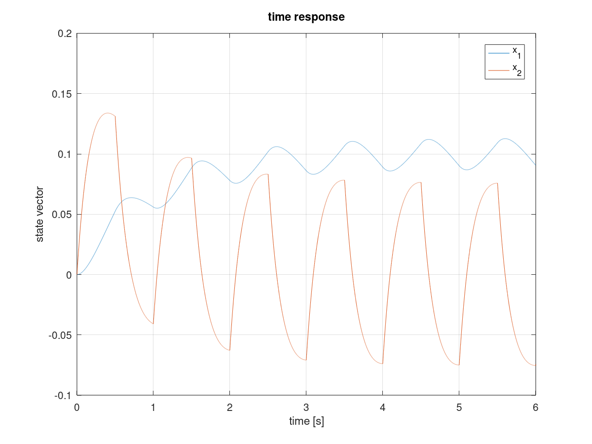
上記のシステムの解。状態変数の初期値は \( \boldsymbol x_0 = \begin{bmatrix} 1 \\ 1 \end{bmatrix} \)、入力は一定値の \( u(t) = 1 \) とする

プログラム（オイラー法）

octave:1> type -q observer_sim.m
clear all

A = [0 1; -5 -6];
B = [0; 1];
C = [1 0];
if false
  D = 0;
end

pkg load control

assert(det(obsv(A, C)) != 0, "system is NOT observable")
assert((det(obsv(A, C)) != 0) == (rank(obsv(A, C)) == size(A)(1)))

Aast = A';
Bast = C';
Cast = B';

F = place(ss(Aast, Bast, Cast), [-7, -8]);
L = F';

dt = 0.001; % [s]
sim_time = 0:dt:6;

u = 1;

i = 1;
for t = sim_time
  if t == 0
    x = [1; 1];
    y = C*x;
    x_1(i) = x(1);
    x_2(i) = x(2);

    xhat = [0; 0];
    yhat = C*xhat;
    xhat_1(i) = xhat(1);
    xhat_2(i) = xhat(2);
  else
    dx = A*x + B*u;
    x = x + dx*dt;
    y = C*x;
    x_1(i) = x(1);
    x_2(i) = x(2);

    dxhat = A*xhat + B*u - L*(yhat - y);
    xhat = xhat + dxhat*dt;
    yhat = C*xhat;
    xhat_1(i) = xhat(1);
    xhat_2(i) = xhat(2);
  end
  i = i + 1;
end

csvwrite("observer_simout.csv", [sim_time', x_1', x_2', xhat_1', xhat_2'])

octave:2> observer_sim

In [1]: %cat observer_visual.py
import pandas as pd
import matplotlib.pyplot as plt

result = pd.read_csv('observer_simout.csv', header=None, names=['time', 'x_1', 'x_2', 'xhat_1', 'xhat_2'])

plt.clf(); plt.grid()
plt.plot(result.time, result.x_1, ls=':', label=r'$ x_1 $')
plt.plot(result.time, result.x_2, ls=':', label=r'$ x_2 $')
plt.plot(result.time, result.xhat_1, alpha=0.6, label=r'$ \hat x_1 $')
plt.plot(result.time, result.xhat_2, alpha=0.6, label=r'$ \hat x_2 $')
plt.legend(loc='best')
plt.xlabel('time [s]'); plt.ylabel('state vector')
plt.title('time response')
plt.savefig('fig_observer_simout.png')

In [2]: %run observer_visual.py

（オブザーバの状態変数の初期値は \( \hat{\boldsymbol x}_0 = \begin{bmatrix} 0 \\ 0 \end{bmatrix} \) としている）

実行結果

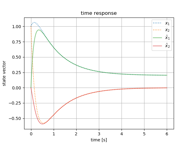
（∴ 設計したオブザーバが状態を推定できていることがわかる）

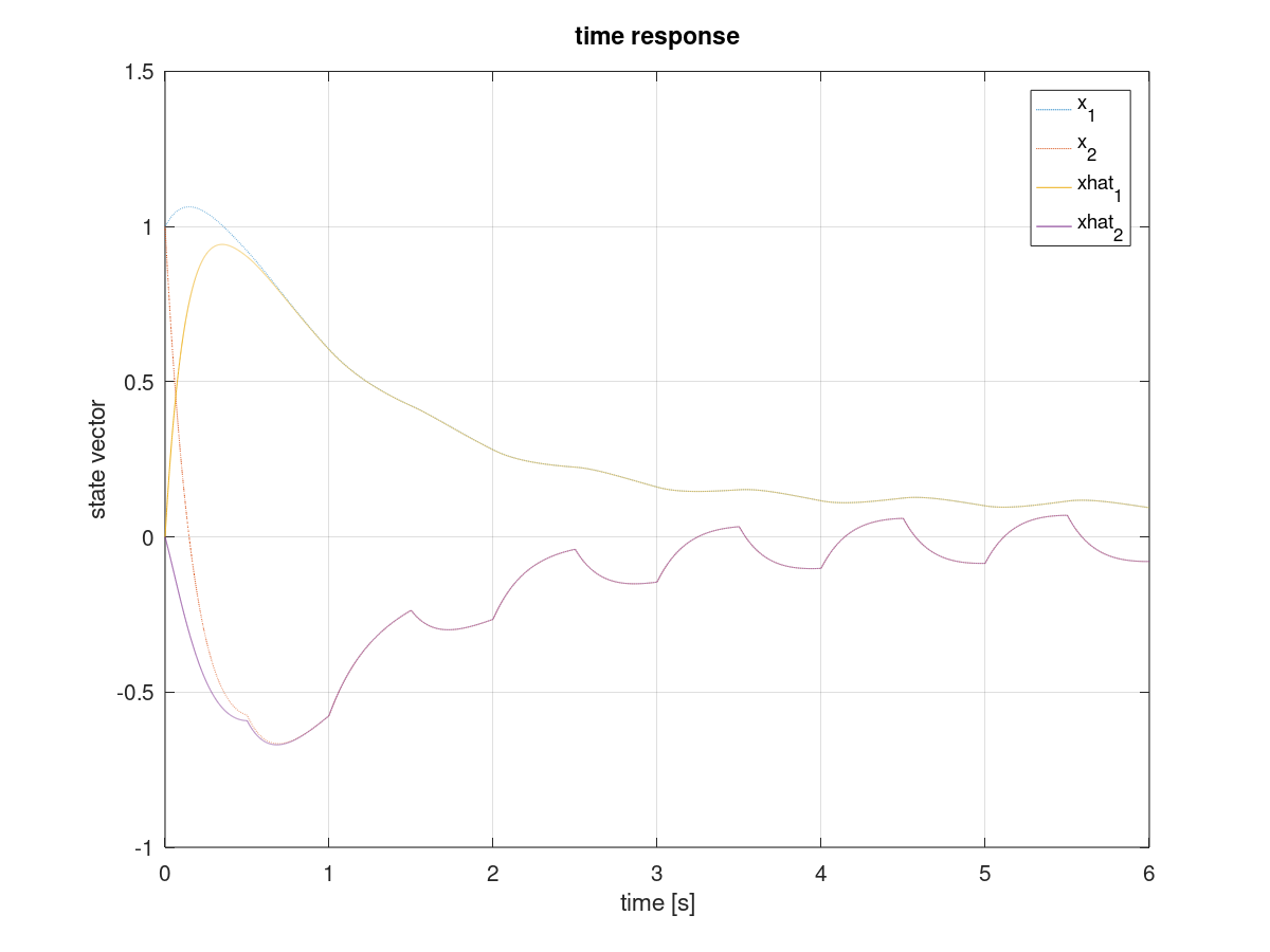
同じシステムに対して、入力 \( u(t) \) を矩形波とする

プログラム

octave:1> type -q observer_sim2.m
clear all

A = [0 1; -5 -6];
B = [0; 1];
C = [1 0];
if false
  D = 0;
end

pkg load control

assert(det(obsv(A, C)) != 0, "system is NOT observable")
assert((det(obsv(A, C)) != 0) == (rank(obsv(A, C)) == size(A)(1)))

Aast = A';
Bast = C';
Cast = B';

F = place(ss(Aast, Bast, Cast), [-7, -8]);
L = F';

dt = 0.001; % [s]
sim_time = 0:dt:6;

i = 1;
for t = sim_time
  if mod(t, 1) > 0.5
    u = 0;
  else
    u = 1;
  end
  if t == 0
    x = [1; 1];
    y = C*x;
    x_1(i) = x(1);
    x_2(i) = x(2);

    xhat = [0; 0];
    yhat = C*xhat;
    xhat_1(i) = xhat(1);
    xhat_2(i) = xhat(2);
  else
    dx = A*x + B*u;
    x = x + dx*dt;
    y = C*x;
    x_1(i) = x(1);
    x_2(i) = x(2);

    dxhat = A*xhat + B*u - L*(yhat - y);
    xhat = xhat + dxhat*dt;
    yhat = C*xhat;
    xhat_1(i) = xhat(1);
    xhat_2(i) = xhat(2);
  end
  i = i + 1;
end

clf
plot(sim_time, x_1, ":", sim_time, x_2, ":")
hold
plot(sim_time, xhat_1, sim_time, xhat_2)
grid on
legend("x_1", "x_2", "xhat_1", "xhat_2")
xlabel("time [s]"); ylabel("state vector")
title("time response")
print("fig_observer_simout2.png", "-dpng")

octave:2> observer_sim2

シミュレーション結果

倒立振子

考えているシステム（系）

（座標系は、右手座標系）

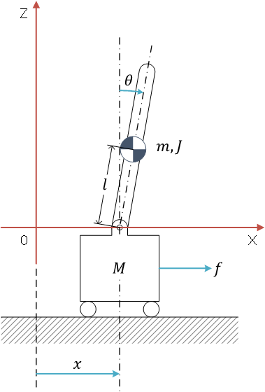倒立振子のパラメータ \( m \) [kg] 振り子の質量 \( J \) [kgm2] 振り子の質量中心（重心）まわりの慣性モーメント \( l \) [m] 振り子の回転軸から質量中心までの距離 \( M \) [kg] 台車の質量 （振り子と台車ともに、粘性抵抗係数 \( \mu \) は考慮していない） 倒立振子の変数 \( \theta \) [rad] 振り子の姿勢（角度） \( x \) [m] 台車の位置 \( f \) [N] 台車の駆動力（直接発生できるとする） （振り子の関節トルク \( \tau \) は発生することができない）

（解析力学より）ラグランジュの運動方程式\[ \frac{d}{dt}\left( \frac{\partial L}{\partial \dot{q}} \right) - \frac{\partial L}{\partial q} = Q - \frac{\partial F}{\partial \dot{q}} \]

F は散逸エネルギー（散逸関数）。粘性摩擦を考慮していないので（粘性摩擦係数 \( \mu = 0 \)）、散逸エネルギーの項は無い\[ \frac{d}{dt}\left( \frac{\partial L}{\partial \dot{q}} \right) - \frac{\partial L}{\partial q} = Q \]

Q は一般化力（制御でいえば入力）。q は一般化座標（ベクトル（ベクトルで微分））

L (Lagrangian) は、運動エネルギー（の総和）からポテンシャルエネルギー（の総和）を引いたもの\[ L = T - U \]

振り子の運動エネルギー。振り子の重心の位置\[ x_g = x + l\sin(\theta),\quad z_g = l\cos(\theta) \]重心の速度（位置を微分して速度）\[ \dot{x}_g = \dot{x} + l\dot{\theta}\cos(\theta),\quad \dot{z}_g = l\dot{\theta}\sin(\theta) \]並進運動の運動エネルギー\[ \begin{align} \frac{1}{2}m v^2 &= \frac{1}{2}m\left( \sqrt{{\dot{x}_g}^2 + {\dot{z}_g}^2} \right)^2 \\ &= \frac{1}{2}m\left( {\dot{x}_g}^2 + {\dot{z}_g}^2 \right) \\ &= \frac{1}{2}m\left( \left( \dot{x} + l\dot{\theta}\cos(\theta) \right)^2 + \left( l\dot{\theta}\sin(\theta) \right)^2 \right) \\ &= \frac{1}{2}m\left(\dot{x}^2 + 2\dot{x}l\dot{\theta}\cos(\theta) + \left( l\dot{\theta}\cos(\theta) \right)^2 + \left( l\dot{\theta}\sin(\theta) \right)^2 \right) \\ &= \frac{1}{2}m\left( \dot{x}^2 + 2\dot{x}l\dot{\theta}\cos(\theta) + l^2\dot{\theta}^2\cos^2(\theta) + l^2\dot{\theta}^2\sin^2(\theta) \right) \\ &= \frac{1}{2}m\left( \dot{x}^2 + 2\dot{x}l\dot{\theta}\cos(\theta) + l^2\dot{\theta}^2\left( \cos^2(\theta) + \sin^2(\theta) \right) \right) \\ &= \frac{1}{2}m\left( \dot{x}^2 + 2\dot{x}l\dot{\theta}\cos(\theta) + l^2\dot{\theta}^2 \right) \end{align} \]振り子の回転運動の運動エネルギー\[ \frac{1}{2}J\dot{\theta}^2 \]

運動エネルギーの総和 T\[ \begin{align} T &= \frac{1}{2}M\dot{x}^2 + \frac{1}{2}m\left( \dot{x}^2 + 2\dot{x}l\dot{\theta}\cos\theta + l^2\dot{\theta}^2 \right) + \frac{1}{2}J\dot{\theta}^2 \\ &= \frac{1}{2}M\dot{x}^2 + \frac{1}{2}m\dot{x}^2 + m\dot{x}l\dot{\theta}\cos\theta + \frac{1}{2}m l^2\dot{\theta}^2 + \frac{1}{2}J\dot{\theta}^2 \\ &= \frac{1}{2}(M + m)\dot{x}^2 + m\dot{x}l\dot{\theta}\cos\theta + \frac{1}{2}(ml^2 + J)\dot{\theta}^2 \end{align} \]

ポテンシャルエネルギー U\[ U = mg z_g = mg l\cos\theta \]

ラグランジュ関数 L\[ \begin{align} L &= T - U \\ &= \left( \frac{1}{2}(M + m)\dot{x}^2 + m\dot{x}l\dot{\theta}\cos\theta + \frac{1}{2}(ml^2 + J)\dot{\theta}^2 \right) - mg l\cos\theta \end{align} \]

θ を一般化座標として\[ \frac{\partial L}{\partial\theta} = -m\dot{x}l\dot{\theta}\sin\theta + mgl\sin\theta \]\[ \begin{align} \frac{d}{dt}\left( \frac{\partial L}{\partial \dot{\theta}} \right) &= \frac{d}{dt}\left( m\dot{x}l\cos\theta + (ml^2 + J)\dot{\theta} \right) \\ &= \frac{\partial (m\dot{x}l\cos\theta)}{\partial \dot{x}}\frac{d\dot{x}}{d t} + \frac{\partial (m\dot{x}l\cos\theta)}{\partial\theta}\frac{d\theta}{dt} + (ml^2 + J)\ddot{\theta} \\ &= m\ddot{x}l\cos\theta - m\dot{x}l\dot{\theta}\sin\theta + (ml^2 + J)\ddot{\theta} \end{align} \]\[ \begin{align} \frac{d}{dt}\left( \frac{\partial L}{\partial \dot{\theta}} \right) - \frac{\partial L}{\partial\theta} &= m\ddot{x}l\cos\theta - m\dot{x}l\dot{\theta}\sin\theta + (ml^2 + J)\ddot{\theta} + m\dot{x}l\dot{\theta}\sin\theta - mgl\sin\theta \\ &= m\ddot{x}l\cos\theta + (ml^2 + J)\ddot{\theta} - mgl\sin\theta \end{align} \]

同様に x を一般化座標として\[ \frac{\partial L}{\partial x} = 0 \]\[ \begin{align} \frac{d}{dt}\left( \frac{\partial L}{\partial \dot x} \right) &= \frac{d}{dt}\left( (M + m)\dot{x} + m l\dot{\theta}\cos\theta \right) \\ &= (M + m)\ddot{x} + \frac{\partial (m l\dot{\theta}\cos\theta)}{\partial \dot{\theta}}\frac{d \dot{\theta}}{dt} + \frac{\partial (m l\dot{\theta}\cos\theta)}{\partial \theta}\frac{d \theta}{dt} \\ &= (M + m)\ddot{x} + m l\ddot{\theta}\cos\theta - m l\dot{\theta}^2\sin\theta \end{align} \]

倒立振子の運動方程式（２本の連立微分方程式）\[ \left\{ \begin{align} & m\ddot{x}l\cos\theta + (ml^2 + J)\ddot{\theta} - mgl\sin\theta = 0 \\ & (M + m)\ddot{x} + m l\ddot{\theta}\cos\theta - m l\dot{\theta}^2\sin\theta = f \end{align} \right. \]

線形化（運動方程式の線形近似）（θ が十分に小さいとき、マクローリン展開の\[ \begin{align} \sin(\theta) &= \theta - \frac{1}{3!}\theta^3 + \frac{1}{5!}\theta^5 - \cdots \approx \theta \\ \cos(\theta) &= 1 - \frac{1}{2!}\theta^2 + \frac{1}{4!}\theta^4 - \cdots \approx 1 \end{align} \]高次の項を無視することができる）\[ \left\{ \begin{align} & m\ddot{x}l + (ml^2 + J)\ddot{\theta} - mgl\theta = 0 \\ & (M + m)\ddot{x} + m l\ddot{\theta} - m l\dot{\theta}^2\theta = f \end{align} \right. \]

さらに、（振り子の角度）\( \theta \approx 0 \) なだけではなく、その角速度 \( \dot\theta \approx 0 \) も成り立っていると仮定すると（２本目の方程式の左辺の第３項を消去できる）\[ \left\{ \begin{align} & m\ddot{x}l + (ml^2 + J)\ddot{\theta} - mgl\theta = 0 \\ & (M + m)\ddot{x} + m l\ddot{\theta} = f \end{align} \right. \]

\( \ddot x \)、\( \ddot\theta \) について連立方程式を解く

(%i1) solve([m*xddot*l + (m*l^2 + J)*thddot - m*g*l*th = 0, (M + m)*xddot + m*l*thddot = f], [xddot, thddot])$

(%i2) tex(%);

もともと２階の微分方程式だったものを、１階の微分方程式として書き直す\[ \left\{ \begin{align} &\frac{d}{dt} x = \dot x \\ &\frac{d}{dt}\theta = \dot\theta \\ &\frac{d}{dt}\dot x \left( = \ddot x \right) = -{{g\,l^2\,m^2\,\theta-f\,l^2\,m-J\,f}\over{\left(M\,l^2+J\right)\,m+J\,M}} \\ &\frac{d}{dt}\dot\theta \left(= \ddot\theta \right) = {{\left(g\,l\,m^2+M\,g\,l\,m\right)\,\theta-f\,l\,m}\over{\left(M\,l^2+J\right)\,m+J\,M}} \end{align} \right. \]

（外力）f はシステムへの入力。変数 f を含む項と含まない項とに分ける\[ \left\{ \begin{align} &\frac{d}{dt} x = \dot x \\ &\frac{d}{dt}\theta = \dot\theta \\ &\frac{d}{dt}\dot x = -{{g\,l^2\,m^2\,\theta}\over{\left(M\,l^2+J\right)\,m+J\,M}} + {{l^2\,m+J}\over{\left(M\,l^2+J\right)\,m+J\,M}}\,f \\ &\frac{d}{dt}\dot\theta = {{\left(g\,l\,m^2+M\,g\,l\,m\right)\,\theta}\over{\left(M\,l^2+J\right)\,m+J\,M}} - {{l\,m}\over{\left(M\,l^2+J\right)\,m+J\,M}}\,f \end{align} \right. \]

θ は変数（振り子の姿勢）\[ \left\{ \begin{align} &\frac{d}{dt} x = \dot x \\ &\frac{d}{dt}\theta = \dot\theta \\ &\frac{d}{dt}\dot x = -{{g\,l^2\,m^2}\over{\left(M\,l^2+J\right)\,m+J\,M}}\,\theta + {{l^2\,m+J}\over{\left(M\,l^2+J\right)\,m+J\,M}}\,f \\ &\frac{d}{dt}\dot\theta = {{g\,l\,m\,\left(m+M\right)}\over{\left(M\,l^2+J\right)\,m+J\,M}}\,\theta - {{l\,m}\over{\left(M\,l^2+J\right)\,m+J\,M}}\,f \end{align} \right. \]

行列の形で連立方程式を整理して、以下の状態方程式を得る\[ \frac{d}{dt} \begin{bmatrix} x \\ \theta \\ \dot{x} \\ \dot{\theta} \end{bmatrix} = \begin{bmatrix} 0 & 0 & 1 & 0 \\ 0 & 0 & 0 & 1 \\ 0 & -{{g\,l^2\,m^2}\over{\left(M\,l^2+J\right)\,m+J\,M}} & 0 & 0 \\ 0 & {{g\,l\,m\,\left(m+M\right)}\over{\left(M\,l^2+J\right)\,m+J\,M}} & 0 & 0 \end{bmatrix}\begin{bmatrix} x \\ \theta \\ \dot{x} \\ \dot{\theta} \end{bmatrix} + \begin{bmatrix} 0 \\ 0 \\ {{l^2\,m+J}\over{\left(M\,l^2+J\right)\,m+J\,M}} \\ - {{l\,m}\over{\left(M\,l^2+J\right)\,m+J\,M}} \end{bmatrix}f \]

（状態ベクトルとして \( \boldsymbol{x} = \begin{bmatrix} x & \theta & \dot{x} & \dot{\theta} \end{bmatrix}^{\mathsf{T}} \) を選んでいる）

倒立振子の制御とシミュレーション

システムの出力は台車の位置 \( x(t) \) と振り子の角速度 \( \dot\theta(t) \)\[ \boldsymbol y(t) = \begin{bmatrix} 1 & 0 & 0 & 1 \end{bmatrix}\boldsymbol x(t) \]として、オブザーバを構成して状態フィードバック制御を行う（→ 併合系）

プログラム

octave:1> type -q inv_pendulum_sim.m
clear all

g = 9.8; % [m/s^2]
m = 0.3; % [kg]
l = 0.4; % [m]
J = (1/12)*m*l^2; % [kg m^2]
M = 0.7; % [kg]

alpha = (M*l^2 + J)*m + J*M;
A = [0 0 1 0; 0 0 0 1; 0 -((g*l^2*m^2)/alpha) 0 0; 0 (g*l*m*(m + M))/alpha 0 0];
B = [0; 0; (l^2*m + J)/alpha; -((l*m)/alpha)];
C = [1 0 0 1];
if false
  D = 0;
end

pkg load control

assert(det(ctrb(A, B)) != 0, "system is NOT controllable")
assert((det(ctrb(A, B)) != 0) == (rank(ctrb(A, B)) == size(A)(1)))
assert(det(obsv(A, C)) != 0, "system is NOT observable")
assert((det(obsv(A, C)) != 0) == (rank(obsv(A, C)) == size(A)(1)))

Aast = A';
Bast = C';
Cast = B';
L = place(ss(Aast, Bast, Cast), [-9, -9, -9, -9])';

Q = eye(4);
R = 1;
F = lqr(A, B, Q, R);

x0 = [0.6; 0.6; 0.6; 0.6];
xhat0 = [0; 0; 0; 0];

xbar0 = [x0; xhat0];
Abar = [A -B*F; L*C A-B*F-L*C];

dt = 0.001; % [s]
sim_time = 0:dt:10;

i = 1;
for t = sim_time
  xbar = expm(Abar*t)*xbar0;
  x_1(i) = xbar(1); x_2(i) = xbar(2); x_3(i) = xbar(3); x_4(i) = xbar(4);
  xhat_1(i) = xbar(5); xhat_2(i) = xbar(6); xhat_3(i) = xbar(7); xhat_4(i) = xbar(8);
  i = i + 1;
end

csvwrite("inv_pendulum_simout.csv", [sim_time', x_1', x_2', x_3', x_4', xhat_1', xhat_2', xhat_3', xhat_4'])

octave:2> inv_pendulum_sim

In [1]: %cat inv_pendulum_visual.py
import pandas as pd
import matplotlib.pyplot as plt

result = pd.read_csv('inv_pendulum_simout.csv', header=None, names=['time', 'x_1', 'x_2', 'x_3', 'x_4', 'xhat_1', 'xhat_2', 'xhat_3', 'xhat_4'])

plt.clf(); plt.grid()
plt.plot(result.time, result.x_1, ls=':', label=r'$ x_1 $')
plt.plot(result.time, result.x_2, ls=':', label=r'$ x_2 $')
plt.plot(result.time, result.x_3, ls=':', label=r'$ x_3 $')
plt.plot(result.time, result.x_4, ls=':', label=r'$ x_4 $')
plt.plot(result.time, result.xhat_1, alpha=0.6, label=r'$ \hat{x}_1 $')
plt.plot(result.time, result.xhat_2, alpha=0.6, label=r'$ \hat{x}_2 $')
plt.plot(result.time, result.xhat_3, alpha=0.6, label=r'$ \hat{x}_3 $')
plt.plot(result.time, result.xhat_4, alpha=0.6, label=r'$ \hat{x}_4 $')
plt.legend(loc='best')
plt.xlabel("time [s]"); plt.ylabel("state vector")
plt.title("time response")
plt.savefig('fig_inv_pendulum_simout.png')

from math import sin, cos
import numpy as np

if True: # adhoc
    l = 0.4 # [m]

frame = 0
for t in np.arange(0, result.time.max(), 0.1):
    plt.clf()
    ax = plt.subplot(1, 1, 1)
    ax.grid()
    ax.set_xlim([-0.1, 1.8]); ax.set_ylim([-0.02, 0.42])
    ax.set_aspect('equal')
    row = result[result.time.round(3) == round(t, 3)]
    assert len(row) == 1, 'error!'
    x = float(row.x_1)
    theta = float(row.x_2)
    ax.plot([x, (x + l*sin(theta))], [0, l*cos(theta)], label=r'$ \vec{x} $')
    ax.scatter(x, 0)
    if False: # observer
        x = float(row.xhat_1)
        theta = float(row.xhat_2)
        ax.plot([x, (x + l*sin(theta))], [0, l*cos(theta)])
        ax.scatter(x, 0)
    ax.set_title('%2.1f'%t + ' [s]')
    ax.set_xlabel('X [m]'); ax.set_ylabel('Z [m]');
    plt.legend(loc='best')
    plt.savefig('fig_inv_pendulum-' + '%02d'%frame  + '.png')
    frame += 1

if True: # make animation
    import os
    os.system('convert -delay 10 -loop 0 fig_inv_pendulum-??.png fig_inv_pendulum.gif')

In [2]: %run inv_pendulum_visual.py

（制御とシミュレーションには Octave、結果の可視化には Python と ImageMagick を利用）

シミュレーション結果

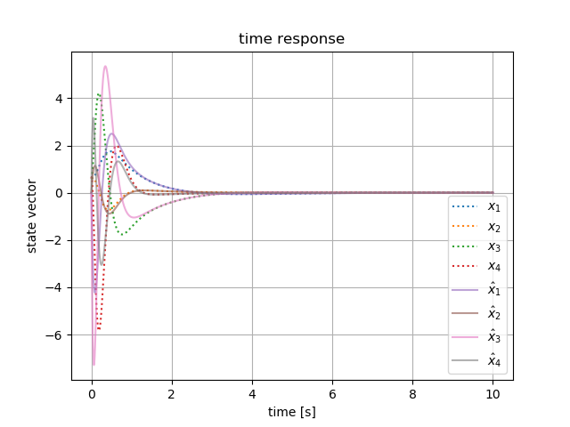（* シミュレーション開始直後に振り子が大きな運動をしているあたりでは、実際の現象とシミュレーションとは一致していないと考えられる（\( \theta \) と \( \dot\theta \) が十分に小さいという仮定をおいて、非線形な微分方程式を線形化しているため））

教科書

• 森泰親, 演習で学ぶ現代制御理論 新装版, 森北出版

参考文献

• 別府 伸耕, 第4章 2輪車の操縦士を数式で表す カルマン・フィルタのプログラミングⅢ 現代制御理論の基礎, トランジスタ技術, ＣＱ出版社, 2019年7月号
• 足立　修一, 6　状態空間表現, MATLABによる 制御工学, 東京電機大学出版局
• 佐藤和也, 下本陽一, 熊澤典良 : はじめての現代制御理論, 講談社

© 2022 Tadakazu Nagai