永井 忠一 2019.8.17
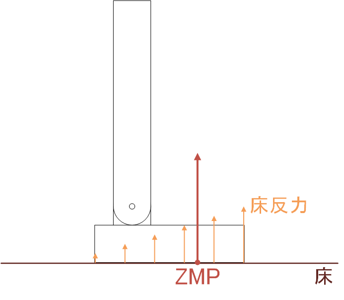
床反力の中心点
|
バランスが取れているときは、ZMPが支持多角形のほぼ中央にある。転倒しているときには、ZMPが支持多角形の縁に達して、その縁を中心にして回転している。ZMPをできるだけ支持多角形の中央にある状態にするのが、バランス制御の基本的な戦略になる。
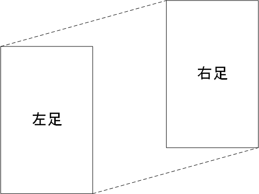
支持多角形
 |
ZMPは支持多角形の領域の外に出ることはない。
外積(cross product)\[ \boldsymbol{\tau}=\boldsymbol{p}\times\boldsymbol{f} \]
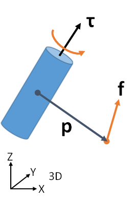
モーメント=位置×力\[ \begin{bmatrix} \tau_x \\ \tau_y \\ \tau_z \end{bmatrix}=\begin{bmatrix} x \\ y \\ z \end{bmatrix}\times\begin{bmatrix} f_x \\ f_y \\ f_z \end{bmatrix}=\begin{bmatrix} yf_{z}-zf_{y} \\ zf_{x}-xf_{z} \\ xf_{y}-yf_{x} \end{bmatrix} \]
(右手座標系)
3次元の1成分が0になったと考える\[ \boldsymbol{\tau}=\boldsymbol{p}\times\boldsymbol{f} \]
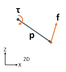
モーメント=位置×力\[ \begin{bmatrix} 0 \\ \tau_y \\ 0 \end{bmatrix}=\begin{bmatrix} x \\ 0 \\ z \end{bmatrix}\times\begin{bmatrix} f_x \\ 0 \\ f_z \end{bmatrix}=\begin{bmatrix} 0 \\ zf_{x}-xf_{z} \\ 0 \end{bmatrix} \]\[ \tau=\tau_y=zf_x-xf_z \]
簡単な例
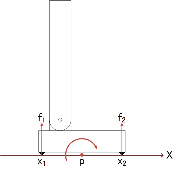
ZMPまわりのモーメント(の水平成分)は0\[ \begin{align} f_{1}(p-x_{1})-f_{2}(x_{2}-p)&=0 \\ f_{1}p-f_{1}x_{1}-f_{2}f_{2}+f_{2}p&=0 \\ (f_1+f_2)p&=f_{1}x_{1}+f_{2}x_{2} \\ p&=\frac{f_{1}x_{1}+f_{2}x_{2}}{f_1+f_2} \end{align} \]
式の確認。全体重がつま先に集中している場合、かかとに作用している力f1=0、つま先だけにf2がかかる\[ p=\frac{0x_{1}+f_{2}x_{2}}{0+f_2}=x_2 \]ZMPはつま先に一致する
市販されている6軸力センサーの例(株式会社レプトリノ)[http://www.leptrino.co.jp/P_CFS.html]
6軸力センサーで計測される値: Fx, Fz(床からの垂直方向の力), τ(Y軸回りのモーメント)
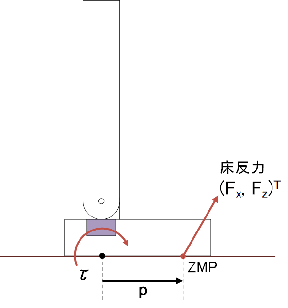
ZMPの計算\[ \begin{align} -\tau&=F_{z}p \\ p&=-\frac{\tau}{F_z} \end{align} \](モーメント[Nm]/力[N]で)位置の次元の量になる。-τのマイナスは回転軸の方向
(実際には、6軸力センサーは足の裏に付いていない)
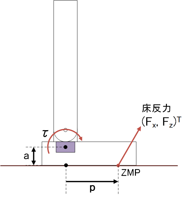
(6軸力センサーを取り付けてある)かかとの高さを考慮したZMPの計算\[ p=\frac{-\tau-aF_x}{F_z} \]
(上記は片足のZMP)
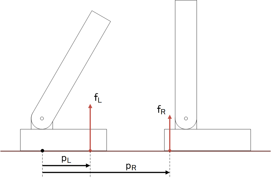
右足と左足それぞれについてZMPを計算して、それを力で配分することによって全体のZMPを計算する\[ p=\frac{f_R}{f_R+f_L}p_R+\frac{f_L}{f_R+f_L}p_L \]
テーブル台車モデルで定式化(簡単なモデルで近似)
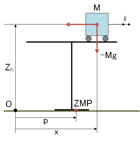
ZMPまわりに重力と台車の加速度が作り出すモーメントが0\[ \tau=(x-p)Mg-Z_{h}M\ddot{x}=0 \](ZMPまわりのモーメントは0)
ZMP方程式の導出(pに関して解く)\[ \begin{align} (x-p)Mg-Z_{h}M\ddot{x}&=0 \\ xMg-pMg-Z_{h}M\ddot{x}&=0 \\ -pMg&=-xMg+Z_{h}M\ddot{x} \\ -p&=\frac{-xMg+Z_{h}M\ddot{x}}{Mg} \\ -p&=-x+\frac{Z_{h}\ddot{x}}{g} \\ p&=x-\frac{Z_{h}}{g}\ddot{x} \end{align} \]
ZMP方程式の意味
ZMP方程式を変形\[ \begin{align} p&=x-\frac{Z_{h}}{g}\ddot{x} \\ -\frac{Z_{h}}{g}\ddot{x}&=p-x \\ \ddot{x}&=-\frac{g}{Z_h}(p-x) \\ \ddot{x}&=\frac{g}{Z_h}(x-p) \end{align} \]
台車(重心)の加速度\[ \ddot{x}=\frac{9.8}{0.98}(0.4-0)=4\,\mathrm{m/s^2} \]
ZMP方程式は重心の運動xからZMPの位置pを求める式。本当に行いたいのは、ZMPを与えてxを求めたい。求めたいのは未知数の重心軌道x
| ZMP | → | \( \boxed{ p=x-\frac{Z_{h}}{g}\ddot{x} } \) | → | 重心軌道x |
ZMPはあらかじめ決定しておく(一歩を何秒ぐらいで歩いてほしいか、一歩をどれくらいの距離で動いてほしいか)
連続だったZMP方程式を離散化する\[ p_i=x_i-\frac{Z_h}{g}\ddot x_i \]Δtは、たとえば5ms間隔。ΔtごとのZMP位置を考えて、Δtごとの重心位置を計算したい。
\( \ddot{x} \)を置き換える。加速度を位置の差分で表現する\[ \ddot{x_i}=\frac{1}{\Delta t}(v_{i+1}-v_i)=\frac{1}{\Delta t}(\frac{x_{i+1}-x_i}{\Delta t}-\frac{x_{i}-x_{i-1}}{\Delta t})\]
速度の差分は加速度。さらに、速度は位置の差分から計算できる。
式を整理してまとめる\[ \ddot x_i=\frac{1}{\Delta t^2}(x_{i-1}-2x_{i}+x_{i+1}) \](加速度の近似式)
\( \ddot x_i \)はxで表現できるので、これをZMP方程式に代入して、整理する。\[ \begin{align} p_i&=x_i-\frac{Z_h}{g}\frac{1}{\Delta t^2}(x_{i-1}-2x_{i}+x_{i+1}) \\ p_i&=\left(-\frac{Z_h}{g\Delta t^2}\right)x_{i-1}+\left(1+2\frac{Z_h}{g\Delta t^2}\right)x_i+\left(-\frac{Z_h}{g\Delta t^2}\right)x_{i+1} \end{align} \]
g, Zh, Δtはすべて定数。得られた、離散化されたZMP方程式\[ p_i=ax_{i-1}+bx_{i}+cx_{i+1} \](a, b, cはまとめられた定数)
知りたいのは重心の位置x、ZMPの位置pは与えられている。これを解くためには、未知数が3つで、既知の値がpだけなのでこれだけでは解けない。
方程式を並べる。たとえば、時刻0から時刻99まで\[ p_0=ax_0+bx_0+cx_1 \\ p_1=ax_0+bx_1+cx_2 \\ p_2=ax_1+bx_2+cx_3 \\ \vdots \\ p_{98}=ax_{97}+bx_{98}+cx_{99} \\ p_{99}=ax_{98}+bx_{99}+cx_{99} \]
これをベクトルと行列(マトリクス)で書き直す\[ \begin{bmatrix} p_0 \\ p_1 \\ p_2 \\ \vdots \\ p_{98} \\ p_{99} \end{bmatrix}=\begin{bmatrix} a+b & c & & & & \\ a & b & c & & & \\ & a & b & c & & \\ & & \ddots & \ddots & \ddots & \\ & & & a & b & c \\ & & & & a & b+c \end{bmatrix}\begin{bmatrix} x_0 \\ x_1 \\ x_3 \\ \vdots \\ x_{98} \\ x_{99} \end{bmatrix} \]
こう書いてしまえば線形代数の問題になる \[ \boldsymbol p=M\boldsymbol x \](pは100次元のZMPベクトル、xは100次元の重心ベクトル、100x100の大きな係数行列M)これもZMP方程式(重心軌道とZMPの関係式)
ZMP方程式がこう書かれたのであれば、逆行列を求めれば与えられたZMPから重心軌道xが求められる\[ \boldsymbol x=M^{-1}\boldsymbol p \](ZMPから重心軌道を得る)
産総研の梶田先生が公開されているコード「BasicGaitGen」を使わせていただきました。m(_o_)m
Octaveを起動して「tridiagonal_demo」を実行
|
与えている目標ZMPの軌跡
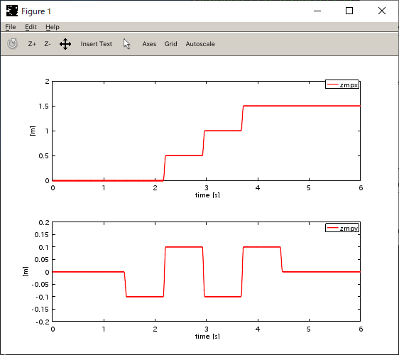
(処理ごとに「pause」しているので、プロンプトから何かキーを押下)
行列(三重対角行列とその逆行列)の可視化
|
| M | M-1 |
|---|---|
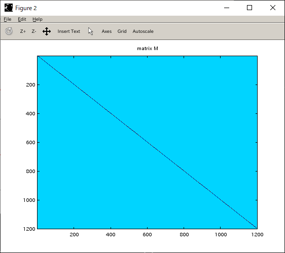 | 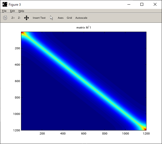 |
重心の計算
|
ZMPと重心(の床面投影点)をプロット
| X軸 | Y軸 |
|---|---|
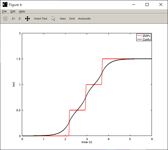 | 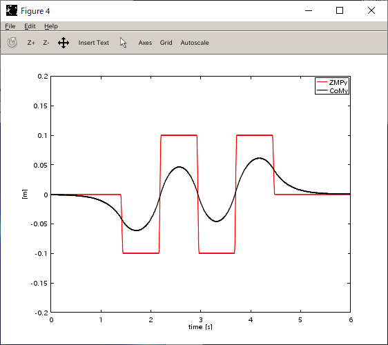 |
《積み残し》
《積み残し》
《積み残し》
Momentが0となる点(床反力の圧力中心点)
(計算ZMP、「(計算上の)計画上のゼロモーメントポイント」について)《今後》
(振り子は、「しんし」とも読む)
 |
|
重心高さ h を一定に保つ。脚長 l は可変(ただし、脚の長さは有限)
(\( h = \text{const.} \) は、過剰拘束)《積み残し》
作図プログラム
| Python |
|---|
|
微分方程式\[ \begin{align} \frac{ma}{mg} = \frac{m\ddot x}{mg} &= \frac{x}{h} \\ \frac{\ddot x}{g} &= \frac{x}{h} \\ \ddot x &= \frac{g}{h}x \end{align} \]
「\( \ddot x = \frac{g}{h}x \)」を解く(ode2() 関数を利用)
| Maxima |
|---|
|
得られた、一般解\[ x = C_1 e^{\sqrt\frac{g}{h}t} + C_2 e^{-\sqrt\frac{g}{h}t} \]
初期条件を用いて任意定数を決定する。(t = 0 のとき)「初期位置 x0、初期速度 v0」として、C1, C2 を求める
| Maxima |
|---|
|
初期位置が「x0 = 0」(原点)、初期速度が「v0 = 0」(静止)の場合の C1, C2 を、それぞれ確認
| Maxima | |
|---|---|
|
|
(ic2() 関数を利用)
| Maxima |
|---|
|
位相平面(位相面)、位相線図

軌道エネルギー《積み残し》
Capture Point《積み残し》
Convergent Component of Motion (CCM)とDivergent Component of Motion (DCM)《積み残し》
作図プログラム
| Python |
|---|
|
問題設定。線形倒立振子、定常状態(定常歩行)
(定常的な)足踏み運動の周期 T [s] を求める
| Maxima |
|---|
|
(find_root() 関数を利用して)求めた数値解は、およそ 1.899 秒
答えを図示。重心の運動の軌跡

作図プログラム
| Python |
|---|
|
問題設定。4足歩行ロボット
支持多角形(足裏が点ならば、2脚支持脚、2脚遊脚で、線分になる)\[ y = Bx\]目標ZMP\[ y_\mathrm{ZMP} = Bvt \]ZMP方程式\[ y_\mathrm{ZMP} = y_\mathrm{CG} - \frac{h}{g}\ddot y_\mathrm{CG} \]
重心軌道を求める微分方程式\[ Bvt = y_\mathrm{CG} - \frac{h}{g}\ddot y_\mathrm{CG} \]
2階微分方程式の一般解
| Maxima |
|---|
|
重心位置\[ y_\mathrm{CG}(t) = C_1\exp\left(\sqrt\frac{g}{h}t\right) + C_2\exp\left(-\sqrt\frac{g}{h}t\right) + Bvt \]重心速度\[ \dot y_\mathrm{CG}(t) = C_1\sqrt\frac{g}{h}\exp\left(\sqrt\frac{g}{h}t\right) - C_2\sqrt\frac{g}{h}\exp\left(-\sqrt\frac{g}{h}t\right) + Bv \]
境界条件。時刻0で原点に位置する\[ y_\mathrm{CG}(0) = 0 \]4分の1周期で、横方向の速度をゼロ(脚切り替えで、次の軌道と滑らかにつながるようにする)\[ \dot y_\mathrm{CG}(\frac{T}{4}) = 0 \]ここで、T は歩行周期
任意定数を決定する
| Maxima |
|---|
|
重心軌道を計算
| Maxima |
|---|
|
ZMPと重心 yCG の軌道

歩容線図(位相 0, 0.5, 1 のところで、脚切り替え)

重心位置と速度(境界条件に使用した速度の方程式も表示して、検算)

作図プログラム
| Python |
|---|
|
© 2019, 2025 Tadakazu Nagai